F1 Car Demo#
This notebook demonstrates how to set up and run an F1 car simulation using the Flow360 Python API.
The project starts from the geometry and goes through:
meshing using the Snappy Mesher:
setting up the meshing task using
ModularMeshingWorkflow,setting multiple zones to be created for porous media,
generating a surface mesh using snappy
setting up a RANS simulation:
defining operating conditions (freestream speed and car attitude),
setting up physical models (walls, moving ground, rotating wheels, porous media, freestream boundaries),
defining a custom output variable and outputs,
submitting a simulation run through
project.run_case().
Note: The settings in this example are by no means a validation setup; they are crafted to showcase the capabilities of Flow360 and we have intentionally reduced node count and example FC cost. For rigorous validation, modify the settings as needed.
1. Imports#
The next code cell imports the Flow360 Python API and some math helpers that will be reused throughout the notebook.
Specifically, we will:
Import
flow360asfl, which provides access to all high-level API objects (projects, boundary conditions, models, outputs, etc.).Import
cos,sin, andradiansfrom the standardmathmodule to construct moving-ground and rotating-wheel velocities.Import
numpyasnpfor creating arrays of slice positions for post-processing outputs.
[1]:
import flow360 as fl
from math import cos, sin, radians
import numpy as np
from flow360.examples import F1_2025
2. Project Setup#
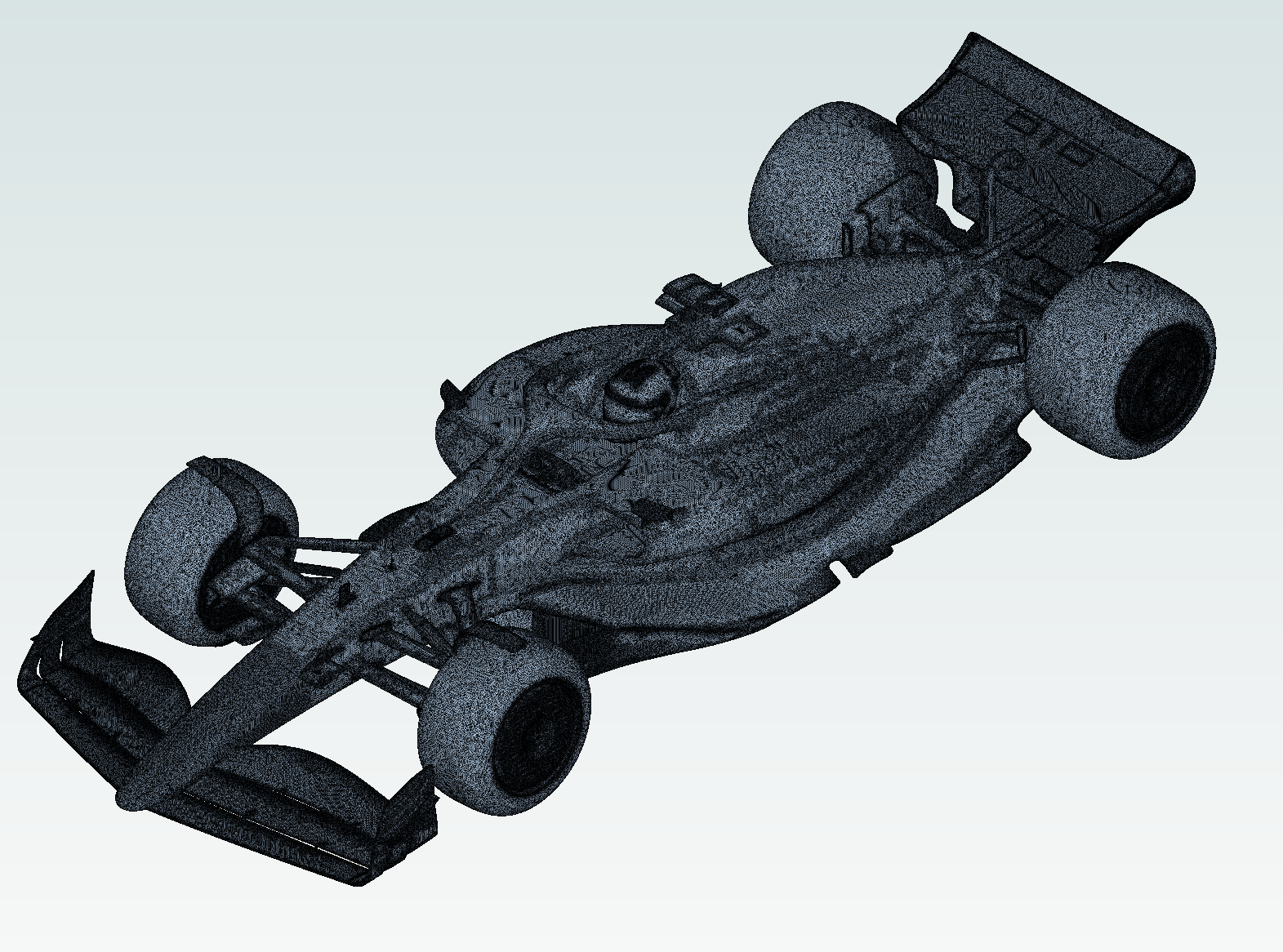
The next code cell creates a Flow360 Project from a geometry. The geometry used is an example Formula 1 car from the 2025 regulations era. It is supplied as a set of component STL files — one per snappy body — which F1_2025.get_files() downloads automatically when the cell runs.
The geometry is grouped for use with snappy. The grouping produces BodyGroups — the equivalent of a searchableSurfaceWithGaps in a snappyHexMesh config — and Surface objects, which are the named faces of those bodies. Bodies are grouped by file, so each component STL file becomes a BodyGroup, and faces are grouped by face into the regions of those bodies. This is handled by the group_bodies_by_tag("groupByFile") and group_faces_by_tag("faceId") calls in the next
cell; no special face-naming convention is required.
The geometry consists of the following files, which you can also download directly:
[ ]:
F1_2025.get_files()

project = fl.Project.from_geometry(
    F1_2025.geometry,
    name="F1 racecar",
    length_unit="m"
)

# uncomment the following line if you already have a project uploaded
# project = fl.Project.from_cloud(project_id="your-project-id")

geometry = project.geometry

geometry.group_bodies_by_tag("groupByFile")
geometry.group_faces_by_tag("faceId")
[15:30:36] INFO: The file (body.stl.zst) is being downloaded, please wait.
[15:30:41] INFO: The file (eb.stl.zst) is being downloaded, please wait.
[15:30:48] INFO: The file (fr-int.stl.zst) is being downloaded, please wait.
[15:30:57] INFO: The file (fr-susp.stl.zst) is being downloaded, please wait.
[15:31:39] INFO: The file (fr-wh.stl.zst) is being downloaded, please wait.
[15:31:43] INFO: The file (fw.stl.zst) is being downloaded, please wait.
[15:31:44] INFO: The file (inflows_outflows.stl.zst) is being downloaded, please wait.
[15:31:53] INFO: The file (rr-int.stl.zst) is being downloaded, please wait.
[15:32:02] INFO: The file (rr-susp.stl.zst) is being downloaded, please wait.
[15:32:49] INFO: The file (rr-wh.stl.zst) is being downloaded, please wait.
[15:32:52] INFO: The file (rw.stl.zst) is being downloaded, please wait.
[15:32:53] INFO: The file (toint-rad.stl.zst) is being downloaded, please wait.
[15:32:57] INFO: The file (tunnel.stl.zst) is being downloaded, please wait.
[15:33:11] INFO: The file (uf.stl.zst) is being downloaded, please wait.
[15:36:49] INFO: Geometry successfully submitted:
                   type        = Geometry
                   name        = F1 racecar
                   id          = geo-b81b051e-4f19-462c-9232-f26e4a39f7ff
                   status      = uploaded
                   project id  = prj-bde06929-783f-4489-8fe1-567801c58404
INFO: Waiting for geometry to be processed.
3. Meshing setup#
In the following cells the meshing task will be set up using the ModularMeshingWorkflow. It needs three parameters to be defined: surface_meshing, volume_meshing and zones.
3.1 Zones#
First the volume zones will be specified. With Snappy the volume zones are defined through the SeedpointVolume objects by providing a point that belongs to that volume. It is recommended that this point does not lay on “round” (integer) coordinates for the snappyHexMesh utility not to break.
In this case three volume zones will be defined:
left hand side radiator
right hand side radiator
fluid
Additionally to the point in mesh, the principal axes are defined to define th coefficients of the PorousMedium later on.
[3]:
rad_lhs = fl.SeedpointVolume(name="rad_lhs",
                             point_in_mesh=[(2040.53452, -405.234, 395.34243)*fl.u.mm],
                             axes=[[19.98, 6.62, 29.21],
                                   [48.076066, -210.05, 14.72]])

rad_rhs = fl.SeedpointVolume(name="rad_rhs",
                             point_in_mesh=[(2040.53452, 405.234, 395.34243)*fl.u.mm],
                             axes=[[19.98, -6.62, 29.21],
                                   [48.076066, 210.05, 14.72]])

fluid = fl.SeedpointVolume(point_in_mesh=[(0.234, 0.18172, 2.1324)*fl.u.m], name="fluid")
3.2 Surface meshing#
The surface mesh is generated using the Snappy mesher. The fl.snappy.SurfaceMeshingParams object controls the surface mesh generation.
3.2.1 General settings#
Firstly general meshing settings (or specifications) will be defined, those include:
``base_spacing``: as an instance of
fl.OctreeSpacingis specified to achieve a fine control over the spacings.snappyHexMesh is an octree based algorithm, meaning that all of the spacings will be the powers of 2 of the master spacing.fl.OctreeSpacingallows to set that master spacing. Individual refinement levels can be then accessed using array indexing (e.g.spacing[1]the master cell divided once), but they can be also defined using numerical values (those values will be cast to the first lower spacing in the octree series).``defaults``:
fl.snappy.SurfaceMeshingDefaultssets the global minimum and maximum spacing, as well as the gap resolution for proximity detection.``smooth_controls``: Laplacian smoothing parameters (
lambda_factor,mu_factor,iterations) to improve surface mesh quality.``castellated_mesh_controls``: controls for the castellated mesh phase, including
resolve_feature_anglewhich determines how sharp edges are captured.
[4]:
surface_defaults = fl.snappy.SurfaceMeshingDefaults(
    min_spacing=8 * fl.u.mm,
    max_spacing=16 * fl.u.mm,
    gap_resolution=0.001 * fl.u.mm, # gaps of this length should be sealed by the mesher, can be specified per face
)

spacing = fl.OctreeSpacing(base_spacing=1 * fl.u.mm)

smooth_controls=fl.snappy.SmoothControls(
    lambda_factor=0.7,
    mu_factor=0.71,
    iterations=5,
)

castellated_mesh_controls=fl.snappy.CastellatedMeshControls(
    resolve_feature_angle=18.0 * fl.u.deg,
)
3.2.2 Uniform surface refinements#
Refinements are defined as a list of objects that override the defaults on specific bodies, regions, or edges in the refinements parameter. As first refinements, to represent the contact patch and the plinths well, fl.UniformRefinement objects with hockey puck like cylinders (plinth_pucks) are defined only for the surface mesher around the plinths to avoid bridging between the ground and the tire.
This is a refinement type applied to a specific volume (if its defined only in the surface mesher, it will not affect the volume mesh directly).
[5]:
with fl.SI_unit_system:
    plinth_pucks = fl.UniformRefinement(
        entities=[
            fl.Cylinder(
                name="fr-lhs-puck",
                center=[200, -800, 10] * fl.u.mm,
                axis=[0, 0, 1],
                outer_radius=150 * fl.u.mm,
                height=15 * fl.u.mm,
            ),
            fl.Cylinder(
                name="fr-rhs-puck",
                center=[200, 800, 10] * fl.u.mm,
                axis=[0, 0, 1],
                outer_radius=150 * fl.u.mm,
                height=15 * fl.u.mm,
            ),
            fl.Cylinder(
                name="rr-lhs-puck",
                center=[3650, -765, -10] * fl.u.mm,
                axis=[0, 0, 1],
                outer_radius=200 * fl.u.mm,
                height=15 * fl.u.mm,
            ),
            fl.Cylinder(
                name="rr-rhs-puck",
                center=[3650, 765, -10] * fl.u.mm,
                axis=[0, 0, 1],
                outer_radius=200 * fl.u.mm,
                height=15 * fl.u.mm,
            ),
        ],
        spacing=0.5 * fl.u.mm,
    )
[15:41:11] INFO: using: SI unit system for unit inference.
3.2.3 Specific surface refinements#
Finally refinements on specific surfaces are defined. Bodies and faces are addressed through the regular geometry registry — geometry["<file>.stl"] returns a body group and geometry["<solid>"] returns a face/Surface (with wildcard support on both). Available types of surface specific refinements include:
fl.snappy.BodyRefinementsets min/max spacing on entire snappy bodies (i.e. whole component files such astunnel.stlorfw.stl); itsbodies=argument takes body groups.fl.snappy.RegionRefinementtargets named faces within a body (e.g. plinth pads, the helmet, individual rim faces); itsregions=argument takesSurfaceentities.fl.snappy.SurfaceEdgeRefinementrefines near sharp edges, with optional angle thresholds and distance-based specification; itsentities=argument accepts either body groups or faces.
[6]:
with fl.SI_unit_system:
    surface_refinements = [
        # --- Tunnel (farfield) — refines the whole tunnel body ---
        fl.snappy.BodyRefinement(
            bodies=[geometry["tunnel.stl"]],
            min_spacing=spacing[-11],
            max_spacing=spacing[-11],
        ),
        # --- Plinth regions  ---
        fl.snappy.RegionRefinement(
            regions=geometry["*plinth*"],
            min_spacing=spacing[1],
            max_spacing=spacing[-2],
        ),
        fl.snappy.SurfaceEdgeRefinement(
            entities=geometry["*plinth*"],
            spacing=[2 * fl.u.mm],
            distances=[5 * fl.u.mm],
        ),
        fl.snappy.SurfaceEdgeRefinement(
            entities=[geometry["tunnel.stl"]],
            spacing=[spacing[-11]],
            distances=[2 * fl.u.mm],
            included_angle=140 * fl.u.deg,
        ),
        # --- Radiator and brake-duct edges ---
        fl.snappy.SurfaceEdgeRefinement(
            entities=[
                geometry["toint-rad-main-*"],
                geometry["body-main-rad-duct"],
                geometry["*-int-brake-duct-*"],
            ],
            spacing=[1 * fl.u.mm],
            distances=[2 * fl.u.mm],
        ),
        # --- Wheels (rims only), helmet, pit ---
        fl.snappy.RegionRefinement(
            regions=[
                geometry["*wh-rim*"],
                geometry["body-helmet"],
                geometry["body-pit"],
            ],
            min_spacing=1 * fl.u.mm,
            max_spacing=4 * fl.u.mm,
        ),
        # --- Body miscellaneous  ---
        fl.snappy.RegionRefinement(
            regions=[geometry["body-misc"]],
            min_spacing=0.5 * fl.u.mm,
            max_spacing=3 * fl.u.mm,
        ),
        # --- Cameras, mirrors, strakes, pillars, vanes, etc. ---
        fl.snappy.RegionRefinement(
            regions=[
                geometry["body-camera"],
                geometry["body-aero-camera"],
                geometry["body-steering-wheel"],
                geometry["uf-strakes"],
                geometry["body-mirror"],
                geometry["rw-pillar"],
                geometry["rr-int-vanes-*"],
                geometry["body-front-af"],
                geometry["body-main-rad-duct"],
            ],
            min_spacing=2 * fl.u.mm,
            max_spacing=8 * fl.u.mm,
        ),
        # --- Suspension ---
        fl.snappy.BodyRefinement(
            bodies=[geometry["fr-susp.stl"], geometry["rr-susp.stl"]],
            min_spacing=4 * fl.u.mm,
            max_spacing=8 * fl.u.mm,
            proximity_spacing=0.5 * fl.u.mm,
        ),
        # --- Front intake winglets & caketins ---
        fl.snappy.RegionRefinement(
            regions=[
                geometry["fr-int-winglet-*"],
                geometry["fr-int-caketin-*"],
            ],
            min_spacing=2 * fl.u.mm,
            max_spacing=8 * fl.u.mm,
            proximity_spacing=0.5 * fl.u.mm,
        ),
        # --- Main body + nose ---
        fl.snappy.RegionRefinement(
            regions=[
                geometry["body"],
                geometry["body-nose"],
            ],
            min_spacing=4 * fl.u.mm,
            max_spacing=8 * fl.u.mm,
        ),
        # --- Front wing ---
        fl.snappy.BodyRefinement(
            bodies=[geometry["fw.stl"]],
            min_spacing=2 * fl.u.mm,
            max_spacing=8 * fl.u.mm,
        ),
        # --- Wheel covers and selected rear-wing elements ---
        fl.snappy.RegionRefinement(
            regions=[
                geometry["*wh-cover-OB*"],
                geometry["rw-ep"],
                geometry["rw-mp"],
                geometry["rw-flap"],
            ],
            min_spacing=2 * fl.u.mm,
            max_spacing=8 * fl.u.mm,
        ),
        # --- Underfloor + diffuser ---
        fl.snappy.RegionRefinement(
            regions=[
                geometry["uf"],
                geometry["diffuser"],
            ],
            min_spacing=2 * fl.u.mm,
            max_spacing=8 * fl.u.mm,
        ),
        # --- Edge refinement on aero surfaces ---
        fl.snappy.SurfaceEdgeRefinement(
            entities=[
                geometry["fw-flap-*"],
                geometry["fw-fine"],
                geometry["fw-ep"],
                geometry["rw-mp"],
                geometry["rw-flap"],
                geometry["diffuser"],
                geometry["uf-strakes"],
                geometry["body-pit"],
            ],
            spacing=1 * fl.u.mm,
            min_elem=3,
            retain_on_smoothing=True,
        ),
        # --- Fine edge refinement on critical aero edges ---
        fl.snappy.SurfaceEdgeRefinement(
            entities=[
                geometry["fw-mp"],
                geometry["rw-gf"],
                geometry["rw-ep"],
                geometry["velocity-*"],
                geometry["eb-exhaust"],
            ],
            spacing=[0.5 * fl.u.mm],
            distances=[1 * fl.u.mm],
            min_elem=10,
            retain_on_smoothing=True,
        )
    ]
INFO: using: SI unit system for unit inference.
The next code cell assembles the fl.snappy.SurfaceMeshingParams object using the defaults and refinements defined above.
[7]:
with fl.SI_unit_system:
    # -----------------------------------------------------------------
    # Assemble surface meshing parameters
    # -----------------------------------------------------------------
    surface_meshing = fl.snappy.SurfaceMeshingParams(
        defaults=surface_defaults,
        refinements=surface_refinements+[plinth_pucks],
        octree_spacing=spacing,
        smooth_controls=smooth_controls,
        castellated_mesh_controls=castellated_mesh_controls
    )
INFO: using: SI unit system for unit inference.
           WARNING: The spacing of 3 mm specified in RegionRefinement will be cast to the first lower refinement in
           the octree series (2 mm).
3.3 Volume meshing#
The volume mesh is generated after the surface mesh. fl.VolumeMeshingParams controls the volume mesh generation, including:
Defaults:
fl.VolumeMeshingDefaultssets the global boundary-layer first-layer thickness and growth rate applied to all walls unless overridden.Refinements: a list of refinement objects that control local mesh density:
fl.PassiveSpacingcontrols howthe boundary layer should be generated (e.g. farfield boundaries). Thetypecan be"unchanged"(do not project) or"projected"(project boundary layer on the surface - for example on tunnel inlet or outlet).fl.BoundaryLayeroverrides the first-layer thickness and growth rate on specific surfaces (e.g. finer layers on aero surfaces, coarser on the ground).fl.UniformRefinementdefines volumetric refinement zones using primitive shapes (fl.Box,fl.Cylinder) to increase resolution in regions of interest (e.g. around the front and rear wings, or under the floor).
Planar face tolerance: controls the tolerance of planar face detection for restoring their planarity..
Gap treatment strength: adjusts boundary layer generation behaviour in narrow gaps. For automotive applications, setting to 1 is recommended.
The code cell below defines volumetric refinement boxes around the front and rear wings, and boundary-layer settings for the ground and aero surfaces.
[8]:
with fl.SI_unit_system:
    # -----------------------------------------------------------------
    # Volume refinements: boxes around regions of interest
    # -----------------------------------------------------------------
    volume_refinements = [
        fl.UniformRefinement(
            entities=[
                fl.Box(
                    name="fr_wing",
                    center=[-650, 0, 250] * fl.u.mm,
                    size=[900, 2100, 600] * fl.u.mm,
                ),
                fl.Box(
                    name="rr_wing",
                    center=[4050, 0, 700] * fl.u.mm,
                    size=[700, 1400, 800] * fl.u.mm,
                ),
            ],
            spacing=16 * fl.u.mm,
        ),
        fl.UniformRefinement(
            entities=[
                fl.Box(
                    name="whole",
                    center=[2000, 0, 750] * fl.u.mm,
                    size=[6500, 2300, 1600] * fl.u.mm,
                )
            ],
            spacing=32 * fl.u.mm,
        ),
    ]

    # -----------------------------------------------------------------
    # Volume meshing parameters
    # -----------------------------------------------------------------
    volume_meshing = fl.VolumeMeshingParams(
        defaults=fl.VolumeMeshingDefaults(
            boundary_layer_first_layer_thickness=0.5 * fl.u.mm,
            boundary_layer_growth_rate=1.2,
            octree_spacing=spacing,
            number_of_boundary_layers=5
        ),
        refinements=[
            # --- Passive spacing on farfield faces ---
            fl.PassiveSpacing(
                faces=[
                    geometry["tunnel-top"],
                    geometry["tunnel-side*"],
                ],
                type="unchanged",
            ),
            fl.PassiveSpacing(
                faces=[
                    geometry["tunnel-inlet"],
                    geometry["tunnel-outlet"],
                ],
                type="projected",
            ),
            # --- Boundary layer on ground ---
            fl.BoundaryLayer(
                faces=[geometry["tunnel-ground"]],
                first_layer_thickness=1 * fl.u.mm,
                growth_rate=1.4,
            ),
            # --- Finer boundary layer on aero surfaces ---
            fl.BoundaryLayer(
                faces=[
                    geometry["fw*"],
                    geometry["rw*"],
                    geometry["uf*"],
                    geometry["diffuser"],
                ],
                first_layer_thickness=0.2 * fl.u.mm,
            ),
            # --- Suspension boundary layer ---
            fl.BoundaryLayer(
                faces=[geometry["*susp*"]],
                first_layer_thickness=0.35 * fl.u.mm,
            ),
            # --- Volume refinements ---
            *volume_refinements,
        ],
        planar_face_tolerance=1e-3,
        gap_treatment_strength=1,
    )
INFO: using: SI unit system for unit inference.
3.4 Full workflow#
Finally, all the meshing components are assembled into a single fl.ModularMeshingWorkflow object:
surface_meshing: thefl.snappy.SurfaceMeshingParamsobject defined in Section 3.2, controlling the snappy surface mesh generation.volume_meshing: thefl.VolumeMeshingParamsobject defined in Section 3.3, controlling boundary layers and volume refinements.zones: afl.CustomZonesobject containing the threeSeedpointVolumeentities (fluid,rad_lhs,rad_rhs) defined in Section 3.1.
This meshing object will later be passed to fl.SimulationParams to define the complete meshing pipeline.
[9]:
meshing = fl.ModularMeshingWorkflow(
    surface_meshing=surface_meshing,
    volume_meshing=volume_meshing,
    zones=[fl.CustomZones(entities=[fluid, rad_lhs, rad_rhs])],
)
           WARNING: The spacing of 3 mm specified in RegionRefinement will be cast to the first lower refinement in
           the octree series (2 mm).
4. Simulation setup#
4.1 Operating condition and time stepping#
The next code cell defines the aerodynamic operating condition (freestream velocity and car attitude) and the steady-state time-stepping strategy with an adaptive CFL:
fl.AerospaceCondition(...)sets the free-stream speed (velocity_magnitude), angle of attackalpha, and sideslipbetausing Flow360’s unit system (fl.u.m / fl.u.s,fl.u.deg). Thealphaangle is set to match the incidence of a wind tunnel that was applied t the geometry to achieve rake.fl.Steady(...)selects a steady-state solver with an adaptive CFL strategy (fl.AdaptiveCFL) and a maximum number of pseudo-time steps.AdaptiveCFLautomatically adjusts the CFL number betweenminandmaxwhile respectingmax_relative_changeandconvergence_limiting_factorto achieve fast but stable convergence.
These operating_condition and time_stepping objects will later be passed into fl.SimulationParams to define the global flow conditions and marching strategy.
[10]:
operating_condition = fl.AerospaceCondition(
    velocity_magnitude=50 * fl.u.m / fl.u.s,
    alpha=-0.273031 * fl.u.deg,
    beta=0.5 * fl.u.deg,
)

time_stepping = fl.Steady(
    CFL=fl.AdaptiveCFL(
        min=0.1,
        max=15000,
        max_relative_change=1,
        convergence_limiting_factor=0.25,
    ),
    max_steps=6000,  # more steps than the mesh-only setup
)
4.2. Boundary Conditions#
The next group of cells defines all boundary-condition models that will be passed into SimulationParams.models:
Wall boundaries for the car body and internal components.
A moving-ground wall to mimic a rolling-road wind tunnel.
Rotating-wall models for all four wheels.
A slip wall on the tunnel top and multiple freestream conditions on inlets, outlets, and ducts.
Each subsection below introduces a specific boundary-condition type and the corresponding code that builds the Flow360 objects.
4.2.1 No-slip Wall Function#
In the following code cell, we define a fl.Wall boundary condition for all solid car surfaces that use a wall-function model:
surfaces=[geometry["fw*"], geometry["rw*"], ...]selects groups of surfaces on the front wing, rear wing, body, underfloor, endplates, suspension, etc., using wildcard patterns over the face names exposed bygroup_faces_by_tag("faceId"). (Wall.surfacesacceptsSurfaceentities, so face-name wildcards are used regardless of how the underlying STL bodies are grouped.)use_wall_function=Truetells Flow360 to use a wall-function approach rather than fully resolving the viscous sublayer.
The resulting wall_model_BC object will be included later in the models list inside SimulationParams.
[11]:
wall_model_BC = [
    fl.Wall(
        surfaces=[
            geometry["fw*"],
            geometry["rw*"],
            geometry["body*"],
            geometry["uf*"],
            geometry["eb*"],
            geometry["fr-int*"],
            geometry["fr-susp*"],
            geometry["rr-int*"],
            geometry["rr-susp*"],
            geometry["diffuser*"],
        ],
        use_wall_function=fl.WallFunction(),
    )
]
4.2.2 Moving Walls#
The next code cell creates a moving ground boundary condition using another fl.Wall object:
surfaces=[geometry["tunnel-ground"]]targets the wind-tunnel floor beneath the car (thetunnel-groundface insidetunnel.stl).velocity=[ ... ] * fl.u.m / fl.u.sspecifies the wall velocity vector in the tunnel frame.The velocity components are constructed from the freestream speed (
50 m/s) combined with the yaw and pitch angles (alpha,beta) usingcos,sin, andradians.
This moving_wall model is later added to the models list so the ground moves with the same speed as the free stream, emulating a rolling road.
[12]:
moving_wall = [
    fl.Wall(
        surfaces=[geometry["tunnel-ground"]],
        use_wall_function=fl.WallFunction(),
        velocity=[
            50 * cos(radians(0.5)) + 50 * cos(radians(-0.273031)),
            50 * sin(radians(0.5)),
            50 * sin(radians(-0.273031)),
        ]
        * fl.u.m
        / fl.u.s,
    )
]
4.2.3 Rotating Walls#
Here we define rotating-wall boundary conditions for the four wheels using a list of fl.Wall objects, each with a fl.WallRotation velocity model:
Each wheel (
front-left,front-right,rear-left,rear-right) is defined as a separatefl.Wallwith asurfaces=[geometry["fr-wh*lhs"], ...]face wildcard that picks up that wheel’s brake-disc, cover, plinth, rim, and tyre surfaces fromfr-wh.stl/rr-wh.stl.fl.WallRotationtakes acenter(rotation center in meters), anaxis(unit vector of the rotation axis), and anangular_velocity(rad/s) to define rigid-body rotation.roughness_height=1 * fl.u.mmsets a simple roughness model on the tire surfaces.
All four wheel walls are collected into the rotating_walls list, which is unpacked later into the models list in SimulationParams.
[13]:
rotating_walls = [
    # --- Rotating front-left wheel ---
    fl.Wall(
        surfaces=[geometry["fr-wh*lhs"]],
        use_wall_function=fl.WallFunction(),
        velocity=fl.WallRotation(
            center=[
                0.20344675860875966,
                -0.7650740158453145,
                0.3592397445075839,
            ]
            * fl.u.m,
            axis=[
                -0.015622695450066178,
                -0.995547991275173,
                0.09295229128344651,
            ],
            angular_velocity=141.50663390275048 * fl.u.rad / fl.u.s,
        ),
        roughness_height=1 * fl.u.mm,
    ),
    # --- Rotating front-right wheel ---
    fl.Wall(
        surfaces=[geometry["fr-wh*rhs"]],
        use_wall_function=fl.WallFunction(),
        roughness_height=1 * fl.u.mm,
        velocity=fl.WallRotation(
            center=[
                0.20344675860875977,
                0.7650740158453145,
                0.3592397445075839,
            ]
            * fl.u.m,
            axis=[
                0.015622695450066141,
                -0.995547991275173,
                -0.0929522912834463,
            ],
            angular_velocity=141.50663390275048 * fl.u.rad / fl.u.s,
        ),
    ),
    # --- Rotating rear-left wheel ---
    fl.Wall(
        surfaces=[geometry["rr-wh*lhs"]],
        use_wall_function=fl.WallFunction(),
        roughness_height=1 * fl.u.mm,
        velocity=fl.WallRotation(
            center=[
                3.6466031503561447,
                -0.742088395684798,
                0.34259442839962195,
            ]
            * fl.u.m,
            axis=[
                0.001488022855271076,
                -0.9993832015999016,
                0.03508564019528322,
            ],
            angular_velocity=142.1293673304936 * fl.u.rad / fl.u.s,
        ),
    ),
    # --- Rotating rear-right wheel ---
    fl.Wall(
        surfaces=[geometry["rr-wh*rhs"]],
        use_wall_function=fl.WallFunction(),
        roughness_height=1 * fl.u.mm,
        velocity=fl.WallRotation(
            center=[
                3.6466031503561456,
                0.7420883956847978,
                0.342594428389622,
            ]
            * fl.u.m,
            axis=[
                -0.001488022855274553,
                -0.9993832015999016,
                -0.0350856401952817,
            ],
            angular_velocity=142.1293673304936 * fl.u.rad / fl.u.s,
        ),
    ),
]
4.2.4 Slip Wall and Freestream Condition#
The next code cell adds a slip-wall boundary on the tunnel top and several freestream boundary conditions on inlets, outlets, and internal ducts:
slip_wall = fl.SlipWall(surfaces=[geometry["tunnel-top"]])creates a slip condition (no normal flow, no shear stress) on the tunnel ceiling.The
freestreamlist contains multiplefl.Freestreamobjects, each targeting the duct inlet/outlet surfaces insideinflows_outflows.stl(velocity-inlet-*,velocity-outlet-*) and, where needed, a prescribed velocity vector.
Both slip_wall and all entries in freestream will be included in the models list to complete the external and internal boundary-condition setup.
[14]:
slip_wall = [fl.SlipWall(surfaces=[geometry["tunnel-top"]])]
freestream = [
    # --- Freestream on tunnel inlet, sides, outlet ---
    fl.Freestream(
        surfaces=[
            geometry["tunnel-inlet"],
            geometry["tunnel-side*"],
            geometry["tunnel-outlet"],
        ]
    ),
    # --- Additional freestream conditions for ducts / exhausts ---
    fl.Freestream(
        surfaces=[geometry["velocity-inlet-exhaust-out"]],
        velocity=[100, 0, 0] * fl.u.m / fl.u.s,
    ),
    fl.Freestream(
        surfaces=geometry["velocity-inlet-fr-int-duct-*-out"],
        velocity=[25.38, 0, 0] * fl.u.m / fl.u.s,
    ),
    fl.Freestream(
        surfaces=geometry["velocity-inlet-rr-int-duct-*-out"],
        velocity=[25.38, 0, 0] * fl.u.m / fl.u.s,
    ),
    fl.Freestream(
        surfaces=[geometry["velocity-outlet-engine-intake-in"]],
        velocity=[21.991020894901634, 0, -21.991020894901634] * fl.u.m / fl.u.s,
    ),
    fl.Freestream(
        surfaces=geometry["velocity-outlet-fr-int-duct-*-in"],
        velocity=[15.36, 0, 0] * fl.u.m / fl.u.s,
    ),
    fl.Freestream(
        surfaces=geometry["velocity-outlet-rr-int-duct-*-in"],
        velocity=[24.93, 0, 0] * fl.u.m / fl.u.s,
    ),
]
4.3 Porous Medium#
The next cell defines a porous-medium model to represent flow resistance through the radiators:
rad_lhsandrad_rhsare volume zones defined in Section 3.1 that correspond to the left-hand and right-hand radiators.Their
axesare set to describe the porous block orientation in space.fl.PorousMedium(...)is then created with:volumes=[rad_lhs, rad_rhs]to apply the model to both radiator volumes.darcy_coefficientandforchheimer_coefficientspecifying the linear and quadratic resistance terms in the porous-medium law.
This porous_medium object is later added to the models list so that radiator pressure losses are captured in the simulation.
[15]:
porous_medium = [
    fl.PorousMedium(
        volumes=[rad_lhs, rad_rhs],
        darcy_coefficient=(3.75e7, 3.75e8, 3.75e8) / fl.u.m**2,
        forchheimer_coefficient=(212.8, 2128, 2128) / fl.u.m,
    )
]
4.4 Custom Output Variable#
The next cell defines a user variable for the non-dimensional velocity, which will be written alongside the standard flow variables.
vel_adim: the velocity vector non-dimensionalised by the free-stream velocity magnitude. It is built with the fl.UserVariable syntax directly from the fl.solution.velocity solver variable and operating_condition.velocity_magnitude.
[16]:
vel_adim = fl.UserVariable(
    name="vel_adim",
    value=[
        fl.solution.velocity[0] / operating_condition.velocity_magnitude,
        fl.solution.velocity[1] / operating_condition.velocity_magnitude,
        fl.solution.velocity[2] / operating_condition.velocity_magnitude,
    ],
)
4.5 Outputs#
The following cell sets up all post-processing outputs for the case:
Slice positions:
x_positions,y_positions, andz_positionsare created withnumpyto define where planes will be cut through the flow field.Surface output: a
fl.SurfaceOutputon all surfaces (geometry["*"]) in ParaView format, writing standard fields such asprimitiveVars,Cp,yPlus, andCfVec.Volume output: a
fl.VolumeOutputthat exports the full 3D field in ParaView format, including built-in solution variables (e.g.vorticity,fl.solution.Cpt_auto) and thevel_adimuser variable.Slice outputs: a
fl.SliceOutputnamed"slices"that contains:X-normal slices (slightly rotated) for each
xinx_positions.Y-normal slices for each
yiny_positions.Z-normal slices for each
zinz_positions.
These outputs are collected in the outputs list, which will be passed to SimulationParams so that all requested data is generated during the run.
[17]:
with fl.SI_unit_system:
    # -----------------------------------------------------------------
    # 4.1 Slice positions
    # -----------------------------------------------------------------
    # These positions define where we will cut the flow field later
    # using SliceOutput (x-normal, y-normal, z-normal planes).
    x_positions = np.arange(-1.1, 5.475, 0.025)
    y_positions = np.arange(-1.1, 1.1, 0.025)
    z_positions = np.arange(-0.05, 1.25, 0.025)

    # Surface output on all surfaces
    outputs = [
        fl.SurfaceOutput(
            surfaces=geometry["*"],
            output_format=["paraview"],
            output_fields=["primitiveVars", "Cp", "yPlus", "CfVec"],
        ),
        # Volume output
        fl.VolumeOutput(
            name="volume",
            output_format=["paraview"],
            output_fields=[
                "primitiveVars",
                "vorticity",
                "residualNavierStokes",
                "residualTurbulence",
                "Cp",
                fl.solution.Cpt_auto,
                "qcriterion",
                vel_adim,
            ],
        ),
        # Slice outputs: x, y, z planes
        fl.SliceOutput(
            name="slices",
            entities=[
                # X-direction slices (slightly rotated around z)
                *[
                    fl.Slice(
                        name=f"slice_x_{i}",
                        normal=(
                            cos(radians(-0.2594)),
                            0,
                            sin(radians(-0.2594)),
                        ),
                        origin=(x, 0, 0),
                    )
                    for i, x in enumerate(x_positions)
                ],
                # Y-direction slices
                *[
                    fl.Slice(
                        name=f"slice_y_{i}",
                        normal=(0, 1, 0),
                        origin=(0, y, 0),
                    )
                    for i, y in enumerate(y_positions)
                ],
                # Z-direction slices
                *[
                    fl.Slice(
                        name=f"slice_z_{i}",
                        normal=(0, 0, 1),
                        origin=(0, 0, z),
                    )
                    for i, z in enumerate(z_positions)
                ],
            ],
            output_format=["paraview"],
            output_fields=[fl.solution.Cpt_auto, "Cp", vel_adim, "vorticity", "qcriterion"],
        ),
    ]
INFO: using: SI unit system for unit inference.
5. Simulation Parameters#
We now build the core SimulationParams object, which collects all pieces defined so far into a single configuration passed to the solver:
Meshing: the
meshingworkflow from Section 3, defining the complete Snappy-based meshing pipeline.Operating condition:
operating_conditionfrom Section 4, defining freestream speed and car attitude.Time-stepping:
time_steppingfrom Section 4, using a steady solver with adaptive CFL.Models: the
modelslist includes:Boundary-condition models:
moving_wall,rotating_walls,slip_wall,freestream, andporous_mediumdefined in Sections 5–6 (unpacked with*in the list).Fluid and turbulence models: a
fl.Fluidobject with aNavierStokesSolverand aKOmegaSSTturbulence model.kappa_MUSCL = 0.33blends central and upwind schemes to reduce numerical dissipation.C_alpha1 = 0.4inKOmegaSSTModelConstantsis chosen to help delay separation.
Custom output variable: the
vel_adimuser variable (Section 4.4) is referenced directly in the output fields, and the total-pressure coefficient uses the built-infl.solution.Cpt_auto. Nouser_defined_fieldsargument is needed.Outputs: the
outputslist from Section 8 (surface, volume, and slice outputs).Reference geometry:
fl.ReferenceGeometrysets the reference moment center, lengths, and area used to compute non-dimensional forces and moments.
The resulting params object is the single input that fully describes the simulation setup for project.run_case.
[18]:
with fl.SI_unit_system:
    params = fl.SimulationParams(
        meshing=meshing,
        operating_condition=operating_condition,
        time_stepping=time_stepping,
        models=[
            # --- Models defined previously ---
            *wall_model_BC,
            *moving_wall,
            *rotating_walls,
            *slip_wall,
            *freestream,
            *porous_medium,
            # --- Fluid + turbulence (k-omega SST) ---
            fl.Fluid(
                navier_stokes_solver=fl.NavierStokesSolver(
                    absolute_tolerance=1e-10,
                    linear_solver=fl.LinearSolver(max_iterations=50),
                    kappa_MUSCL=0.33,
                    low_mach_preconditioner=True,
                ),
                turbulence_model_solver=fl.KOmegaSST(
                    absolute_tolerance=1e-8,
                    linear_solver=fl.LinearSolver(max_iterations=25),
                    equation_evaluation_frequency=4,
                    rotation_correction=True,
                    modeling_constants=fl.KOmegaSSTModelConstants(C_alpha1=0.4),
                ),
            ),
        ],
        outputs=outputs,
        reference_geometry=fl.ReferenceGeometry(
            moment_center=(1.4001, 0, -0.3176),  # reference moment center
            moment_length=(1, 2.7862, 1),  # reference lengths
            area=1.7095,  # reference area
        ),
    )
INFO: using: SI unit system for unit inference.
6. Run Simulation#
The final code cell submits the case to Flow360 using the project.run_case API:
project.run_case(params=params, name="Tutorial F1 Car from Python")sends the fullparamsobject (constructed in Section 5) to the Flow360 service and starts a simulation run.The
nameargument provides a human-readable label for this specific run within the project.
Before executing this cell, you should double-check all previous sections (meshing, BCs, models, outputs, and reference geometry), as running this cell will launch a real simulation in your Flow360 workspace and consume computational resources.
[ ]:
case = project.run_case(
    params=params,
    name="Tutorial F1 Car from Python",
    use_beta_mesher=True
)
[15:41:12] WARNING: The spacing of 3 mm specified in RegionRefinement will be cast to the first lower refinement in
           the octree series (2 mm).
           WARNING: Validation warnings found during local validation:
                   (1) Multiple symmetry plane surfaces have different boundary conditions (Freestream, Wall).
           Please check if this is intended.
INFO:
INFO: Units of output `UserVariables`:
INFO: -------------------------------
INFO: Variable Name | Unit
INFO: -------------------------------
INFO: Cpt_auto_SI | dimensionless
INFO: vel_adim | dimensionless
INFO: -------------------------------
INFO:
[15:41:13] INFO: Selecting beta/in-house mesher for possible meshing tasks.
[15:41:15] INFO: Successfully submitted:
                   type        = Case
                   name        = Tutorial F1 Car from Python
                   id          = case-bd5651a0-1001-4120-9781-a4dee36905c8
                   status      = pending
                   project id  = prj-bde06929-783f-4489-8fe1-567801c58404