Download notebook (.ipynb)

Download script (.py)

SRF with Cube

This notebook demonstrates how to set up a Single Rotating Frame (SRF) simulation with a mesh of a simple cube using snappyHexMesh in Flow360.

Key features demonstrated:

• Integration of snappyHexMesh for surface meshing with Flow360’s new volume mesher

• Definition of rotating zones using the Rotation model

• Setup of boundary conditions for SRF simulations

• Use of the modular meshing workflow with custom zones

Note: The settings in this example are by no means a validation setup; they are crafted to showcase the capabilities of Flow360 and we have intentionally reduced node count and example FC cost. For rigorous validation, modify the settings as needed.

1. Create Project from geometry

The first step is to initialize the Flow360 client and create a project from the geometry file.

Key steps:

• Load libraries: Import flow360 and the example geometry (Cube). The Cube example provides a pre-configured STL file for demonstration purposes — it contains two named solids, cube and farfield.

• Create project: Use fl.Project.from_geometry() to create a project from the CAD file. Specify the length_unit (meters in this case).

• Group bodies and faces: From release 25.10 onward, snappy uses the same conventional grouping mechanism as the other surface meshers. Call geo.group_bodies_by_tag("groupByFile") to expose each input STL file as a body group (here, a single cube.stl body), and geo.group_faces_by_tag("faceId") to expose each named STL solid as an addressable surface (here, geo["cube"] and geo["farfield"]).

import flow360 as fl
from flow360.examples import Cube

fl.Env.preprod.active()

Cube.get_files()

project = fl.Project.from_geometry(
    Cube.geometry, name="SRF Cube", length_unit="m"
)

geo = project.geometry
geo.show_available_groupings(verbose_mode=True)
geo.group_bodies_by_tag("groupByFile")
geo.group_faces_by_tag("faceId")

[06:05:30] INFO: The file (cube.stl) is being downloaded, please wait.

[06:05:48] INFO: Geometry successfully submitted:
                   type        = Geometry
                   name        = SRF Cube
                   id          = geo-8810a17f-5c89-4203-b66d-2f6973408725
                   status      = uploaded
                   project id  = prj-fee2c42f-311f-4e60-8c4f-90f8512d066b
           

           INFO: Waiting for geometry to be processed.

[06:06:11] INFO:  >> Available attribute tags for grouping **faces**:

           INFO:     >> Tag '0': groupByBodyId. Grouping with this tag results in:

           INFO:         >> [0]: cube.stl

           INFO:            IDs: ['cube', 'farfield']

           INFO:  >> Available attribute tags for grouping **edges**:

           INFO:  >> Available attribute tags for grouping **bodies**:

           INFO:     >> Tag '1': groupByFile. Grouping with this tag results in:

           INFO:         >> [0]: cube.stl

           INFO:            IDs: ['cube.stl']

2. Meshing Parameters

The meshing configuration uses Flow360’s modular meshing workflow, which allows you to independently choose surface and volume meshers. This example combines:

• Surface meshing: snappyHexMesh integration via fl.snappy.SurfaceMeshingParams

• Volume meshing: Flow360’s new volume mesher via fl.VolumeMeshingParams

Defining the fluid zone:

The fluid domain must be explicitly defined using a SeedpointVolume:

• point_in_mesh: A list of one or more coordinate points that lie inside the fluid region (e.g., [[10.1435, 0, 0]]). The seed points help the mesher identify which volume is the fluid domain.

• center and axis: Define the center and rotation axis for the volume. These are critical for SRF simulations, as they specify the rotation reference frame. Here, center=(0, 0, 0) and axis=(1, 0, 0) indicate rotation about the x-axis through the origin.

• Convert to zone: Wrap the SeedpointVolume in a CustomZones object to make it available for meshing and physics models.

Surface meshing configuration:

• ``SurfaceMeshingDefaults``: Global surface meshing parameters:

  • min_spacing and max_spacing: Control the surface mesh resolution

  • gap_resolution: Minimum feature size to capture (1 mm)

• ``RegionRefinement``: Refine a specific surface (region) of the geometry. Here it targets geo["cube"] — the cube face exposed by the faceId grouping — to give the wall a finer mesh than the surrounding farfield. Faces are addressed by their STL solid name (geo["<face>"]); bodies are addressed by their file name (geo["<file>.stl"]) and accepted by fl.snappy.BodyRefinement when the refinement should cover the whole body.

• ``SurfaceEdgeRefinement``: Refine the mesh along surface edges to capture sharp features and geometric discontinuities. If this refinement is not used, the edges are not guaranteed to be kept by snappyHexMesh. The spacing parameter (50 mm in this example) controls the mesh size along edges, while distances (2 mm) defines the distance from the edge where this refinement is applied.

Volume meshing configuration:

• ``VolumeMeshingDefaults``: Set boundary layer parameters:

  • boundary_layer_first_layer_thickness: Thickness of the first boundary layer cell (1 mm), which affects near-wall resolution and is important for accurate wall-bounded flow predictions.

• Volume meshing refinements:

  • ``PassiveSpacing``: Preserve the surface mesh spacing on specified faces. Applied to the farfield surface geo["farfield"] with type='unchanged', this prevents the volume mesher from modifying the mesh spacing on the farfield boundary, maintaining the resolution determined by the surface mesher.

  • ``UniformRefinement``: Apply uniform mesh spacing within a defined region. Here, a box region (center at (0.5, 0, 0) with size 3×2×2 m) is refined to 50 mm spacing to ensure adequate resolution around the cube geometry in the near-field region.

Important: When using the new volume mesher, you must set use_beta_mesher=True when running the case (see Section 5).

with fl.SI_unit_system:
    fluid = fl.SeedpointVolume(name="fluid", point_in_mesh=[(10.1435, 0, 0)], center=(0, 0, 0), axis=(1, 0, 0))
    fluid_zone = fl.CustomZones(name="fluid", entities=[fluid])

    meshing_params = fl.ModularMeshingWorkflow(
        surface_meshing=fl.snappy.SurfaceMeshingParams(
            defaults=fl.snappy.SurfaceMeshingDefaults(
                min_spacing=0.5 * fl.u.m, max_spacing=2 * fl.u.m, gap_resolution=1 * fl.u.mm
            ),
            refinements=[
                fl.snappy.RegionRefinement(
                    min_spacing=50 * fl.u.mm, max_spacing=100 * fl.u.mm,
                    regions=[geo["cube"]]
                ),
                fl.snappy.SurfaceEdgeRefinement(
                    spacing=[50 * fl.u.mm],
                    distances=[2 * fl.u.mm],
                    entities=[geo["cube"]]
                )
            ]
        ),
        volume_meshing=fl.VolumeMeshingParams(
            defaults=fl.VolumeMeshingDefaults(boundary_layer_first_layer_thickness=1 * fl.u.mm),
            refinements=[
                fl.PassiveSpacing(
                    faces=[geo["farfield"]],
                    type='unchanged'
                ),
                fl.UniformRefinement(
                    entities=fl.Box(name="box", center=(0.5, 0, 0), size=(3, 2, 2)),
                    spacing=50 * fl.u.mm
                )
            ]
        ),
        zones=[fluid_zone],
    )

           INFO: using: SI unit system for unit inference.

3. Create Rotating Model

In an SRF simulation, the entire computational domain rotates as a rigid body. The Rotation model defines which volumes rotate and at what angular velocity.

Key parameters:

• ``name``: A descriptive name for the rotation model (e.g., "rotating_farfield")

• ``volumes``: List of volumes that rotate. Here, we use the fluid volume defined earlier, which means the entire fluid domain rotates.

• ``spec``: The rotation specification. AngularVelocity(10 * fl.u.rpm) sets the domain to rotate at 10 revolutions per minute about the axis defined in the SeedpointVolume (x-axis through the origin).

Important considerations:

• The rotation axis and center must match those defined in the SeedpointVolume (Section 2) for consistency.

• In SRF simulations, boundary conditions are applied in the rotating frame. For example, a freestream velocity is specified relative to the rotating domain.

• The Rotation model is added to the models list in SimulationParams (Section 4), not as a boundary condition.

with fl.SI_unit_system:
    rotating_farfield = fl.Rotation(
        name="rotating_fluid",
        volumes=[fluid],
        spec=fl.AngularVelocity(50 * fl.u.rpm)
    )

           INFO: using: SI unit system for unit inference.

4. Create SimulationParams

The SimulationParams class consolidates all simulation settings: meshing, physics, boundary conditions, and solver options.

Configuration components:

1. ``meshing``: Reference to the ModularMeshingWorkflow defined in Section 2.

2. ``operating_condition``: Defines the flow conditions:

   • AerospaceCondition(velocity_magnitude=10 * fl.u.m / fl.u.s): Sets a freestream velocity of 10 m/s. In SRF simulations, this velocity is relative to the rotating frame.

3. ``time_stepping``: Steady() indicates a steady-state simulation. For unsteady SRF cases, use Unsteady() with appropriate time step settings.

4. ``models``: List of physics models and boundary conditions:

   • ``Wall``: Applied to the cube surface using geo["cube"]. Each STL solid is exposed as a Surface entity named after that solid, so the cube face is selected directly. No-slip boundary conditions are applied by default.

   • ``Freestream``: Applied to the farfield surface using geo["farfield"]. This sets the farfield boundary condition with the velocity specified in operating_condition.

   • ``rotating_farfield``: The rotation model defined in Section 3. This makes the entire fluid domain rotate.

5. ``reference_geometry``: ReferenceGeometry() enables calculation of reference quantities (forces, moments) for the cube geometry.

Note: The order of models in the list doesn’t matter, but all relevant models must be included.

with fl.SI_unit_system:
    params = fl.SimulationParams(
        meshing=meshing_params, # Previously defined meshing parameters
        operating_condition=fl.AerospaceCondition(velocity_magnitude=10 * fl.u.m / fl.u.s),
        time_stepping=fl.Steady(),
        models=[
            fl.Wall(
                surfaces=[geo["cube"]]
            ),
            fl.Freestream(
                surfaces=[geo["farfield"]]
            ),
            rotating_farfield,
        ],
        reference_geometry=fl.ReferenceGeometry(),
        outputs=[
            fl.SurfaceOutput(
                surfaces=[geo["cube"]],
                output_fields=['CfVec', 'Cf', 'yPlus', 'Cp']
            )
        ]
    )

           INFO: using: SI unit system for unit inference.

5. Run Case

Submit the case to Flow360’s cloud platform using project.run_case().

Key parameters:

• ``params``: The SimulationParams object containing all simulation configuration.

• ``name``: A descriptive name for the case (visible in the Flow360 web interface).

• ``solver_version``: Must match the version used when creating the project to ensure compatibility.

• ``use_beta_mesher=True``: Required when using VolumeMeshingParams (the new volume mesher). This flag tells Flow360 to use the beta meshing pipeline instead of the default mesher.

What happens next:

1. The case is submitted and queued for execution.

2. Flow360 performs surface meshing using snappyHexMesh.

3. Volume meshing is performed using the new volume mesher.

4. The CFD solver runs the simulation.

5. Results are available for download and visualization.

case = project.run_case(params=params, name="SRF cube from Python", use_beta_mesher=True)

           WARNING: The spacing of 50 mm specified in RegionRefinement will be cast to the first lower refinement
           in the octree series (31.25 mm).

           WARNING: The spacing of 100 mm specified in RegionRefinement will be cast to the first lower refinement
           in the octree series (62.5 mm).

           WARNING: The spacing of 50 mm specified in SurfaceEdgeRefinement will be cast to the first lower
           refinement in the octree series (31.25 mm).

           WARNING: The spacing of 50 mm specified in UniformRefinement will be cast to the first lower refinement
           in the octree series (31.25 mm).

[06:06:12] INFO: Selecting beta/in-house mesher for possible meshing tasks.

[06:06:14] INFO: Successfully submitted:
                   type        = Case
                   name        = SRF cube from Python
                   id          = case-cf6239a4-538a-40bf-8e3f-bf1f33e954c4
                   status      = pending
                   project id  = prj-fee2c42f-311f-4e60-8c4f-90f8512d066b
           

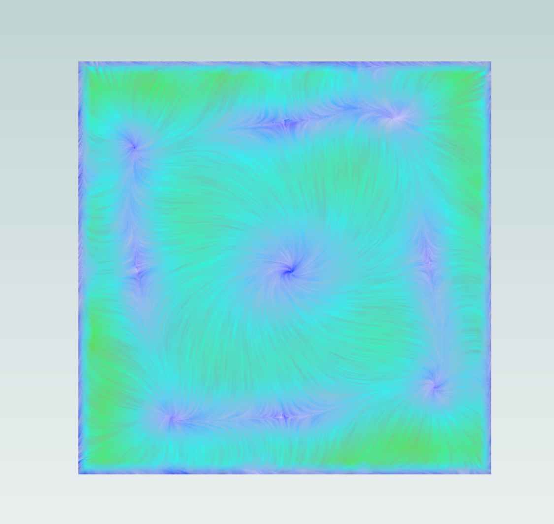
Image showing the friction lines on the front face of the cube, notice there is a swirl component.