Non-Dimensional Outputs#
Note
With the introduction of User Variables, manual dimensionalization of outputs is no longer needed.
When using a User Variable, simply specify what unit system the variable should be output in. The underlying conversion from a non-dimensional output to a dimensional one, follows the same logic that is described below.
In this section, we demonstrate how to compute the dimensional value for the non-dimensional outputs obtained from the non-dimensional Flow360 solver (such as output fields). At the completion of a case, the Flow360 solver generates multiple CSV files and visualization files containing the history of important variables.
The following list shows some commonly used non-dimensional variables in these output files:
Property |
Ref. value for nondim. |
Examples of non-dimensional outputs in Flow360 |
|---|---|---|
Length |
\(L_\text{gridUnit}\) |
|
Density |
\(\rho_\infty\) |
|
Velocity |
\(C_\infty\) |
|
Pressure |
\(\rho_\infty C_\infty^2\) |
|
Temperature |
\(T_\infty\) |
|
Heat Flux |
\(\rho_\infty C_\infty^3\) |
|
BET, Actuator Disk and Porous Media Force |
\(\rho_\infty C_\infty^2 L_\text{gridUnit}^2\) |
force in BET output |
BET, Actuator Disk and Porous Media Moment |
\(\rho_\infty C_\infty^2 L_\text{gridUnit}^3\) |
moment in BET output |
Note
In the above table, all reference values can be accessed through Python API as shown in the Reference Variable Table.
In addition to the forces and moments of BET/Actuator Disk, the non-dimensionalization for all other forces and moments are demonstrated in the Force and Moment Coefficients Section.
To demonstrate how to perform non-dimensionalization on these variables, we use the predefined operating_condition and reference_geometry to obtain these reference values.
For a completed
caseinproject:project.length_unit,case.params.operating_conditionandcase.params.reference_geometrycan be used to access the reference values.case.resultscan be used to access all output results. These results can be downloaded viacase.results.download(...)function in python API or from WebUI. See Python API Guide for more details.
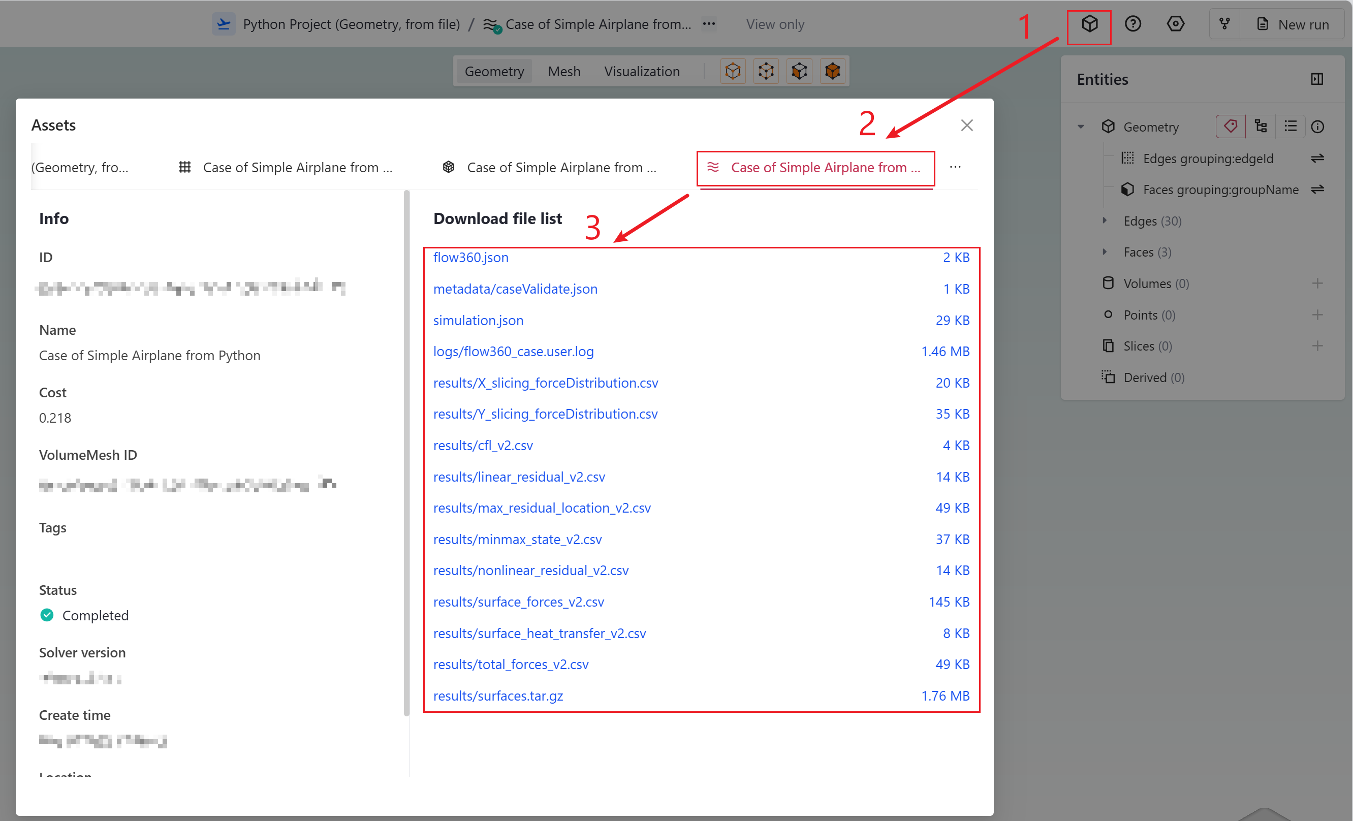
Fig. 7.1.1 Procedures to access case results.#
Example: Output Fields in Visualization Files#
Flow360 solver supports the following visualization output formats:
ParaView (.pvtu)
Tecplot (.szplt)
The export file type as well as the variables exported are set up using different types of Outputs of Python API. These visualization files are compressed in the “surfaces.tar.gz” and “volumes.tar.gz” etc. as shown in the Figure above. The exported data are non-dimensional. Some examples of dimensional conversions are shown below:
Velocity#
Because the reference value of velocity is \(C_\infty\) from Table 7.1.4,
the dimensional velocity in x-direction can be obtained by multiplying the velocityX with the freestream speed of sound.
Assuming the freestream speed of sound is 340 m/s and velocityX is 0.6 in the ParaView/Tecplot file, then the dimensional velocity in x-direction is \(340 \text{ m/s} \times 0.6 = 204 \text{ m/s}\).
Pressure#
The reference value of pressure is \(\rho_\infty C_\infty^2\) from Table 7.1.4.
Assuming the freestream speed of sound is 340 m/s, freestream density is 1.225 kg/m 3 and p is 0.65 in the ParaView/Tecplot file, then the dimensional pressure is \(0.65 \times 1.225 \, \text{kg}/\text{m}^3 \times 340^2 \, \text{m}^2/\text{s}^2 = 92046.5 \, \text{Pa}\).
Node Force Per Unit Area#
nodeForcesPerUnitArea is the total (pressure + friction) force applied at a node divided by the surface area attributed to the given node. It is particularly useful to calculate sectional loading values. If integrated over the whole surface, nodeForcesPerUnitArea would equal the total forces acting on the surface. The reference value to dimensionalize nodeForcesPerUnitArea is the same as for pressure \(\rho_\infty C_\infty^2\).
Skin Friction Coefficient#
As defined, CfVec is the skin friction coefficient vector and Cf is the magnitude of that vector. To calculate the viscous stress on the wall:
The CfVec vector is very useful to locate regions of boundary layer separation. Fully attached flow follows the surface along the streamwise direction, whereas separated flow induces local recirculation.
A strategy to investigate separation is to visualize skin friction in the streamwise direction. For example, consider flow in the x-direction over a wing, regions of negative CfVecX indicate boundary layer separation.
If we set a visualization scale with 3 levels, say -1e-6, 0 and 1e-6 we will have all the negative values be one color and all the positive values be another, hence we can easily find the regions of separated flows on the surface. See the image below:
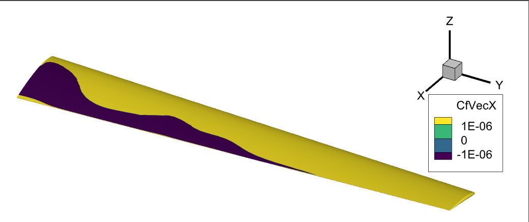
Fig. 7.1.2 The x-component of skin friction coefficient showing the attached (yellow) and separated (dark purple) flow regions on this wing at a high angle of attack.#
The separated flow regions on the surface can also be visualized by using surface streamlines. Because the velocities on the surface are, by definition of a NoSlipWall, equal to 0, the key is to change the surface streamline integration parameters from velocity{X,Y,Z} to CfVec{X,Y,Z}.
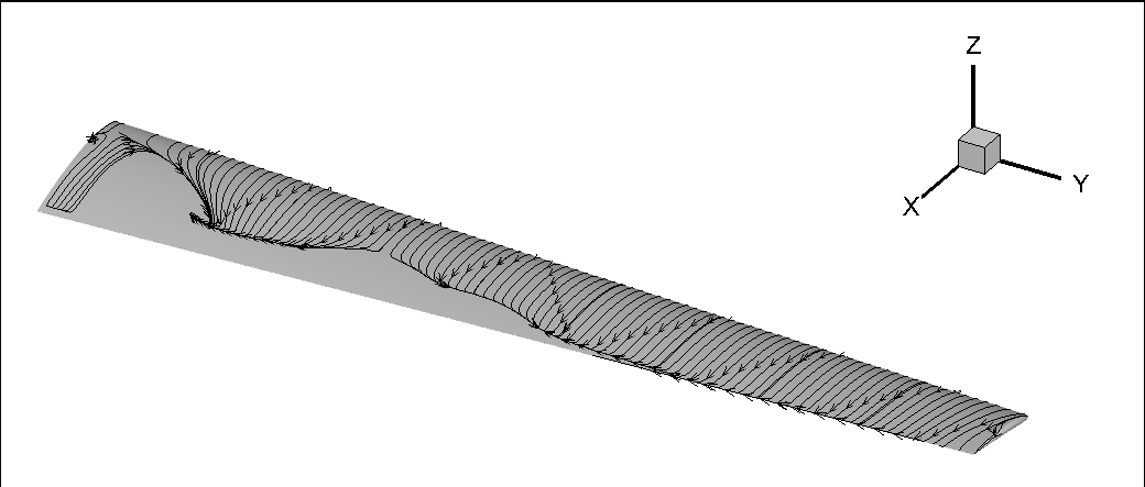
Fig. 7.1.3 Surface streamlines showing recirculation regions.#
Pressure Coefficient#
To calculate the dimensional pressure simply use:
where \(p_\infty \ \text{(N/m$^2$)}\) is the ambient pressure at the farfield.
Total Pressure Coefficient#
By definition total pressure is the sum of static pressure $p$, dynamic pressure $q$, and gravitational head. In most applications we can ignore the gravitational head. Total pressure can also be called stagnation pressure because at a stagnation point the velocity is 0, thus the dynamic pressure $q$ term becomes 0 and the total pressure becomes equal to the static pressure $p$ at that stagnation point.
As shown in equations 26 and 29 in the appendix of this paper, the total pressure coefficient \(C_{pt}\) can be calculated using the following formula:
where the heat capacity ratio \(\gamma= 1.4\) for standard air conditions. The dimensional total pressure can be similarly calculated as with static pressure,
Just like we used CfVecX to visualize the surface separation regions above, we can use \(C_{pt}\) to visualize regions of separation in the flow volume.
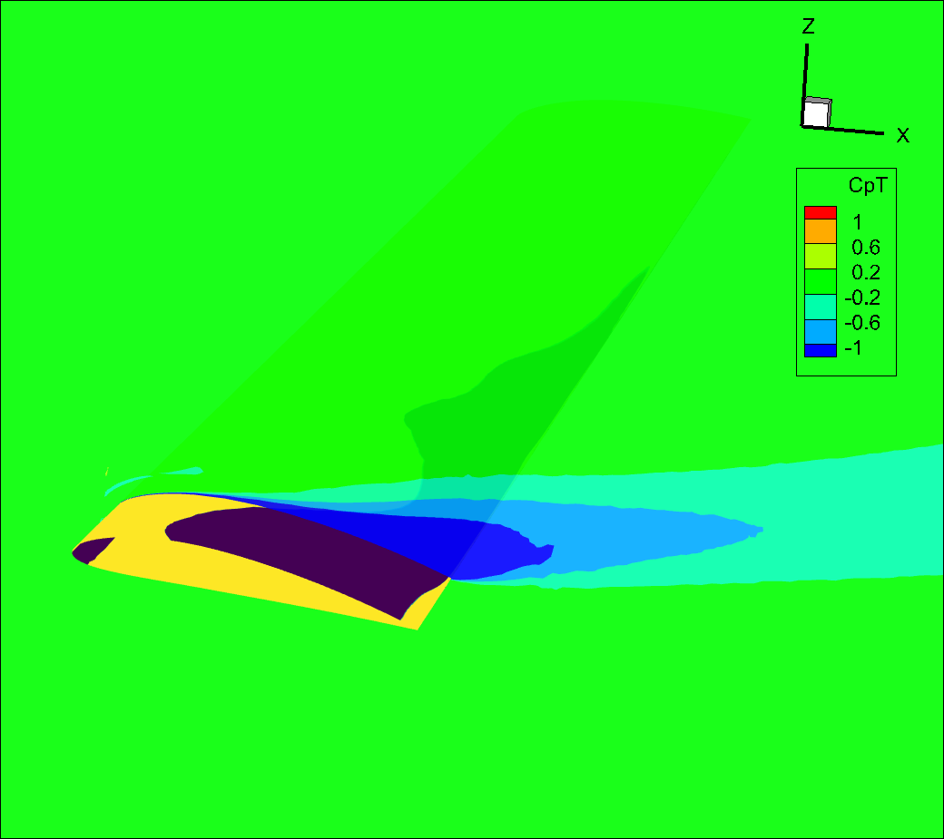
Fig. 7.1.4 Slice of total pressure coefficient showing separation region on a partially stalled wing.#
The \(C_{pt}\) variable is also effective to visualize the boundary layer, if we look at the same slice as above but zoom in on the leading edge, we can see the boundary layer developing.
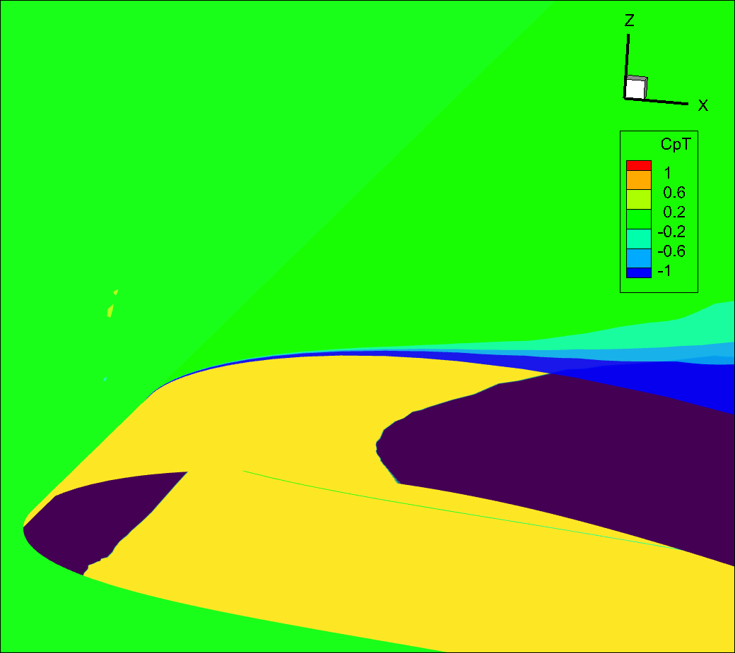
Fig. 7.1.5 Slice of total pressure coefficient showing the growing boundary layer in blue.#
Q-Criterion#
The qcriterion is a very convenient way to visualize vortices in your flowfield. By setting
qcriterion isosurfaces in your volume solution you can easily identify vortices and gain a better understanding of their behavior.
In general, for airplane type simulations, we recommend setting an isosurface value to \(\frac{\text{Mach}^2}{\text{Wing Span}^2}\). For rotor dominated flows, we typically recommend \(\frac{\text{Tip Mach}^2}{\text{Rotor Diameter}^2}\). Depending on the amount of vorticity in your flow you will have to adapt that metric value to best visualize your vortices. A larger isosurface value will only show stronger vortices. Reducing the isosurface value will visualize weaker vortices, showing more flow features but at the risk of cluttering the visualization.
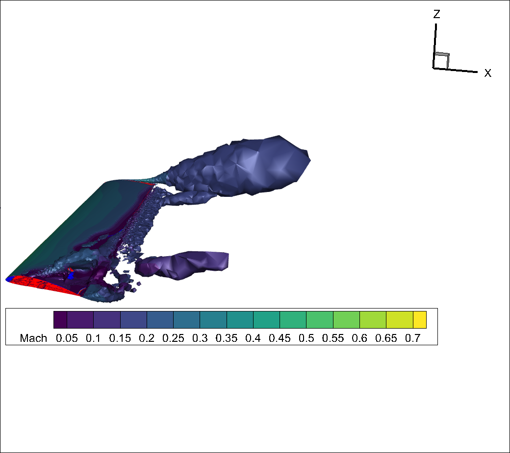
Fig. 7.1.6 qcriterion isosurface showing strong tip vortex and vortices escaping from the separation region.#
You will notice that, for this test case, because the volume mesh is quite coarse the qcriterion isosurface has a very jagged appearance and the vortex structures dissipate quickly.
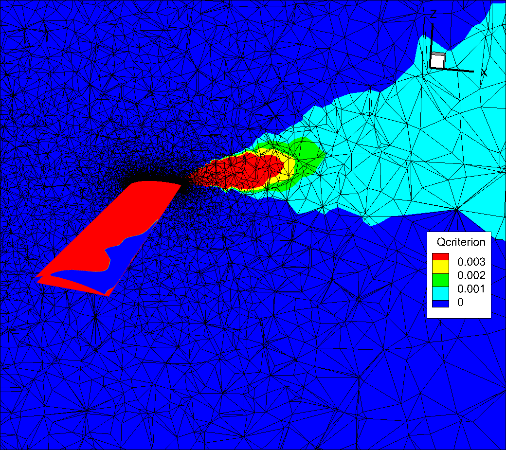
Fig. 7.1.7 Slice showing the volume mesh. Notice how quickly the mesh coarsens as we move away from the wing and how that affects the qcriterion values.#
If we refine the far field substantially by applying a refinement region we can obtain a much smoother qcriterion isosurface showing improved resolution of the vortices escaping from the tip and from the separation bubble.
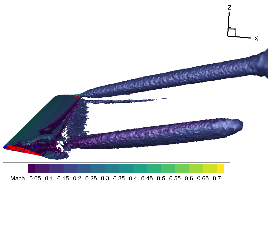
Fig. 7.1.8 qcriterion isosurface on a finer mesh showing strong tip vortex and vortices escaping from the separation region.#
You will notice that now, for this refined volume mesh, the qcriterion isosurface has a much smoother appearance and the vortex structures propagate much further (i.e., are much less dissipative).
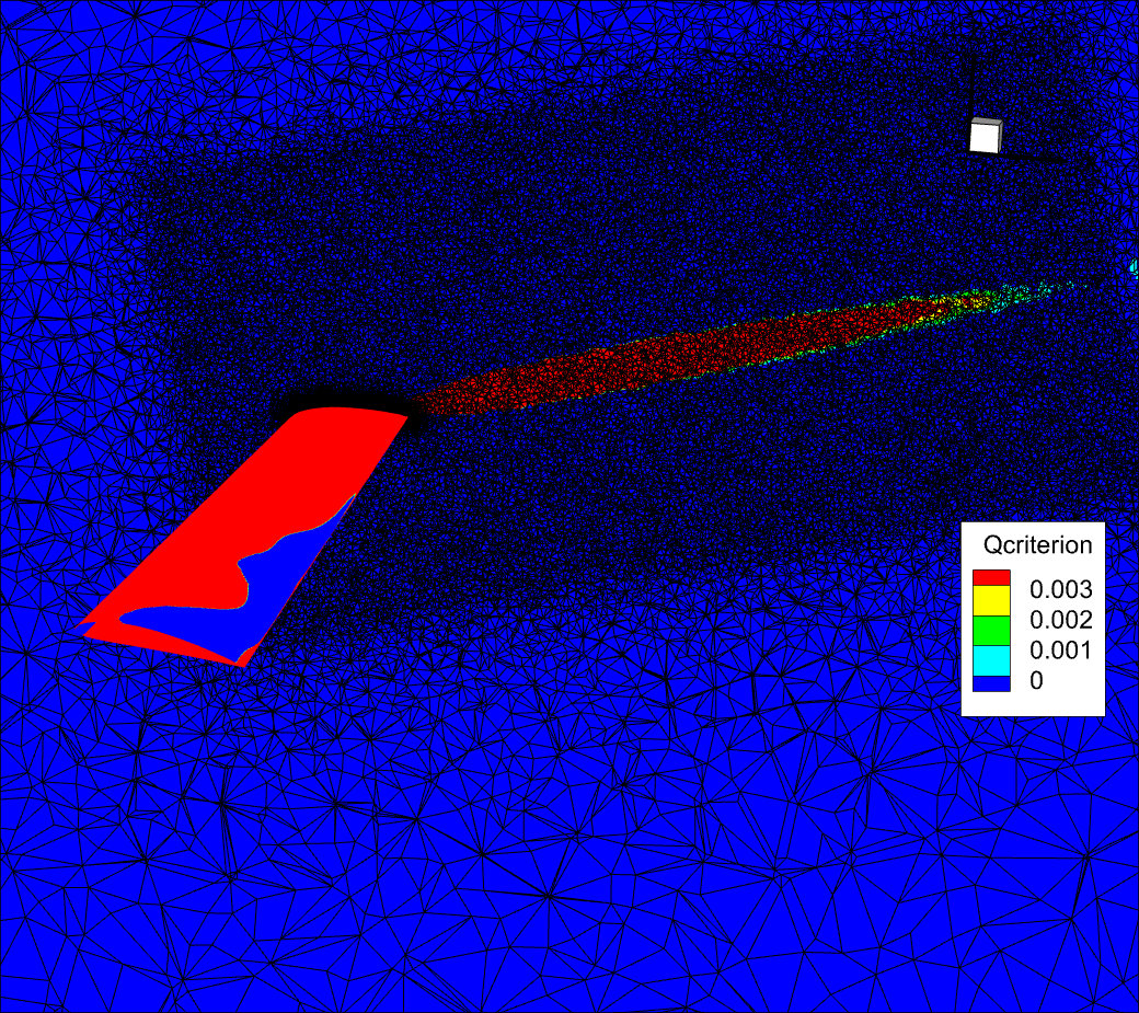
Fig. 7.1.9 Slice showing the volume mesh. Finer volume mesh showing the effect on the qcriterion dissipation.#
For more flow images using the qcriterion to visualize vortices please see:
Example: Actuator Disk Output CSV File#
The Actuator Disk (AD) output file, “actuatorDisk_output_v2.csv”, has the following headers: physical_step, pseudo_step, Disk0_Power, Disk0_Force, Disk0_Moment, Disk1_Power, Disk1_Force, Disk1_Moment ....DiskN_Power, DiskN_Force, DiskN_Moment for the N disks. The data in this
The power column contains the \(C_p\) power coefficient:
Note that the information in the “actuatorDisk_output_v2.csv” file can be accessed using case.results.bet_disks_forces. The following code demonstrates how to obtain the dimensional power of Disk0:
1# The output values are averaged over the last 10% steps
2actuator_disk_output = case.results.actuator_disks.averages
3
4density = case.params.operating_condition.thermal_state.density
5speed_of_sound = case.params.operating_condition.thermal_state.speed_of_sound
6length_unit = project.length_unit
7
8C_p = actuator_disk_output['Disk0_Power']
9power = C_p * density * speed_of_sound**3 * length_unit**2
The Force and Moment columns simply report the constant integrated total force and moment as entered by the user.
Attention
Compared to the commonly used force and moment coefficients, Actuator Disk’s forces and moments use \(C_\infty\) instead of \(U_\text{ref}\) as the reference velocity value for non-dimensionalization.
Example: BET Loading Output CSV File#
The Blade Element Theory (BET) output file, “bet_forces_v2.csv”, contains the time history of the following quantities:
Integrated x-, y-, z-component of non-dimensional forces and non-dimensional moments acted on each disk, represented by “Disk[diskID]_Force_x,_y,_z” and “Disk[diskID]_Moment_x,_y,_z”, respectively. The non-dimensional force is defined as,
(7.1.13)#\[\text{Force}_\text{non-dimensional} = \frac{\text{Force}_\text{physical} \ \text{(N)}}{\rho_\infty C_\infty^2 L_\text{gridUnit}^2}\]and non-dimensional moment as,
(7.1.14)#\[\text{Moment}_\text{non-dimensional} = \frac{\text{Moment}_\text{physical} \ \text{(N$\cdot$m)}}{\rho_\infty C_\infty^2 L_\text{gridUnit}^3}\]where the moment center is the
centerof each disk.Note
The above Force and Moment values are forces and moments acting on the solid. Forces and moments acting on the fluid are the inverse of the above.
Note
The above equations for Force (Eq.(7.1.13)) and Moment (Eq.(7.1.14)) are also applicable to Porous Media forces and moments as reported in the “porous_media_output.csv” file.
Attention
The x-, y-, z-component of Disk[diskID]_Force and Disk[diskID]_Moment is reported in the global inertial reference frame. This reference frame is defined in the mesh file.
Compared to the commonly used force and moment coefficients, BET Disk’s forces and moments use \(C_\infty\) instead of \(U_\text{ref}\) as the reference velocity value for non-dimensionalization.
Sectional thrust coefficient \(C_t\) and sectional torque coefficient \(C_q\) on each blade at several radial locations, represented by “Disk[diskID]_Blade[bladeID]_R[radialID]” with suffix “_Radius” (non-dimensional), “_ThrustCoeff” and “_TorqueCoeff”. The number of radial locations is specified in
nLoadingNodes.Note
\(C_t\) and \(C_q\) are sectional loadings, whereas \(C_T\) and \(C_Q\) are integrated loads of the entire rotor. That is, \(C_t\bigl(r\bigr)=\frac{\text{d}C_T}{\text{d}(r/R)}\) and \(C_q\bigl(r\bigr)=\frac{\text{d}C_Q}{\text{d}(r/R)}\).
The definition of \(C_t\) is,
(7.1.15)#\[C_t\bigl(r\bigr)=\frac{\text{Thrust per unit blade span (N/m)}}{\frac{1}{2}\rho_{\infty}\left((\Omega r)^2\right)\text{chord}_{\text{ref}}}\cdot\frac{r}{R}\]and \(C_q\) is,
(7.1.16)#\[C_q\bigl(r\bigr)=\frac{\text{Torque per unit blade span (N)}}{\frac{1}{2}\rho_{\infty}\left((\Omega r)^2\right)\text{chord}_{\text{ref}} \cdot R}\cdot\frac{r}{R}\]where \(r\) is the dimensional distance between the radial station and the axis of rotation. \(\text{chord}_\text{ref}\) is the dimensional reference chord length. \(R\) is the dimensional radius of the rotor disk.
Important
All the quantities in the right-hand side of Eq.(7.1.13), Eq.(7.1.14), Eq.(7.1.15) and Eq.(7.1.16) are dimensional, which are different from the non-dimensional values in the “bet_forces.csv” file. For example, at the first disk’s first blade’s first radial location \(r=\text{Disk0_Blade0_R0_Radius}\times L_\text{gridUnit}\). The conventions for non-dimensional outputs can be found at Reference values for non-dimensional outputs in Flow360.
Warning
For steady-state simulations with BET models, the resulting \(C_t\) and \(C_q\) are only saved on the first blade, named by “Blade0”. They are written as all zeros for other blades, because all the blades have the same sectional loadings in steady BET Disk simulations. For unsteady BET Line simulations, each blade has its own \(C_t\) and \(C_q\) values.
Here is an example of the header of a “bet_forces.csv” file from a simulation containing two BET disks (assume nLoadingNodes = 20, numberOfBlades = 3 for each disk):
physical_step, pseudo_step,
Disk0_Force_x, Disk0_Force_y, Disk0_Force_z, Disk0_Moment_x, Disk0_Moment_y, Disk0_Moment_z,
Disk0_Blade0_R0_Radius, Disk0_Blade0_R0_ThrustCoeff, Disk0_Blade0_R0_TorqueCoeff,
Disk0_Blade0_R1_Radius, Disk0_Blade0_R1_ThrustCoeff, Disk0_Blade0_R1_TorqueCoeff,
...
Disk0_Blade0_R19_Radius, Disk0_Blade0_R19_ThrustCoeff, Disk0_Blade0_R19_TorqueCoeff,
Disk0_Blade1_R0_Radius, Disk0_Blade1_R0_ThrustCoeff, Disk0_Blade1_R0_TorqueCoeff,
Disk0_Blade1_R1_Radius, Disk0_Blade1_R1_ThrustCoeff, Disk0_Blade1_R1_TorqueCoeff,
...
Disk0_Blade1_R19_Radius, Disk0_Blade1_R19_ThrustCoeff, Disk0_Blade1_R19_TorqueCoeff,
Disk0_Blade2_R0_Radius, Disk0_Blade2_R0_ThrustCoeff, Disk0_Blade2_R0_TorqueCoeff,
Disk0_Blade2_R1_Radius, Disk0_Blade2_R1_ThrustCoeff, Disk0_Blade2_R1_TorqueCoeff,
...
Disk0_Blade2_R19_Radius, Disk0_Blade2_R19_ThrustCoeff, Disk0_Blade2_R19_TorqueCoeff,
Disk1_Force_x, Disk1_Force_y, Disk1_Force_z, Disk1_Moment_x, Disk1_Moment_y, Disk1_Moment_z,
...
...
...
Disk1_Blade2_R19_Radius, Disk1_Blade2_R19_ThrustCoeff, Disk1_Blade2_R19_TorqueCoeff
Note that the information in the “bet_forces_v2.csv” file can be accessed using case.results.bet_disks_forces. The following python example demonstrates how to obtain the dimensional force, moment, sectional thrust, and sectional torque of Disk0:
 1# The output values are averaged over the last 10% steps
 2bet_disks_forces = case.results.bet_forces.averages
 3
 4density = case.params.operating_condition.thermal_state.density
 5speed_of_sound = case.params.operating_condition.thermal_state.speed_of_sound
 6length_unit = project.length_unit
 7
 8force_disk0_x_non_dim = bet_disks_forces["Disk0_Force_x"]
 9moment_disk0_x_non_dim = bet_disks_forces["Disk0_Moment_x"]
10# Compute dimensional Force and Moment on disk0
11force_disk0_x = force_disk0_x_non_dim * density * speed_of_sound**2 * length_unit**2
12moment_disk0_x = moment_disk0_x_non_dim * density * speed_of_sound**2 * length_unit**3
13
14
15# Assuming the index of BETDisk model in params.models is 4
16bet_model = case.params.models[4]
17chord_ref = bet_model.chord_ref
18omega = bet_model.omega
19radius_rotor_disk = bet_model.entities.stored_entities[0].outer_radius
20
21r1 = bet_disks_forces["Disk0_Blade0_R1_Radius"]
22thrust_disk0_blade0_r1_coeff = bet_disks_forces["Disk0_Blade0_R1_ThrustCoeff"]
23torque_disk0_blade0_r1_coeff = bet_disks_forces["Disk0_Blade0_R1_TorqueCoeff"]
24
25# Compute dimensional Thrust and Torque at disk0, blade0 at r1
26thrust_disk0_blade0_r1 = thrust_disk0_blade0_r1_coeff * 0.5 * density * omega**2 \
27   * r1 * length_unit * radius_rotor_disk * chord_ref
28torque_disk0_blade0_r1 = torque_disk0_blade0_r1_coeff * 0.5 * density * omega**2 \
29   * r1 * length_unit * radius_rotor_disk**2 * chord_ref
Example: Aeroacoustic Output CSV File#
The aeroacoustic output file has the name “total_acoustics_v3.csv” which contains the overall aeroacoustic results for all wall patches combined. If AeroacousticOutput.write_per_surface_output has been set to True then “surface_NameOfPatch_acoustics_v3.csv” will also be available for each of the individual wall patches.
Each CSV file contains the following headers: “time, physical_step, observer_0_pressure, observer_1_pressure, … , observer_N_pressure, observer_0_thickness, … , observer_N_thickness, observer_0_loading, … , observer_N_loading”, where N+1 is the total number of observers specified in the aeroacousticOutput section of the case JSON file. The "_pressure" columns provide the acoustic pressure signal at the observer locations and the "_thickness" and "_loading" columns correspond to the thickness and loading noise contributions to the acoustic pressure signal.
The output file contains the non-dimensional acoustic pressure signal as a function of time, where time is the non-dimensional time specified in the first column. The second column is the physical step of the simulation at which the time is observed, assuming constant time step size.
Note
The time of observation is not necessarily contained in the simulation time as it will take a finite amount of time for the acoustic signal to propagate from the solid surfaces to the observers’ locations. As each observer can have a different distance from the solid surface, certain observers will have a proper acoustic signal before other observers at any given time. Consequently, the acoustic signal at each observer is padded with zeros at the beginning and the end of the time history, depending on the validity of the acoustic signal.
Example: Heat Transfer CSV File#
The file “surface_heat_transfer_v2.csv” contains surface integrals of the heat flux computed from non-dimensional quantities. To find the dimensional heat transfer rate, multiply the non-dimensional value by \(\rho_{\infty}C_{\infty}^3 L_\text{gridUnit}^2\).
Note that the information in the “surface_heat_transfer_v2.csv” file can be accessed using case.results.surface_heat_transfer. The following code demonstrates how to obtain the dimensional power of Disk0:
 1# The output values are averaged over the last 10% steps
 2surface_heat_transfer = case.results.surface_heat_transfer.averages
 3
 4density = case.params.operating_condition.thermal_state.density
 5speed_of_sound = case.params.operating_condition.thermal_state.speed_of_sound
 6length_unit = project.length_unit
 7
 8# Assuming the surface name is fluid/Interface_solid
 9heat_flux_no_dim = surface_heat_transfer["fluid/Interface_solid_HeatTransferRate"]
10heat_flux = heat_flux_no_dim * density * speed_of_sound**3 * length_unit**2