7.8. Conjugate Heat Transfer for Cooling Fins

This tutorial will walk you through the process of running a steady-state simulation using a conjugate heat transfer (CHT) solver. By specifying the volume heat source, you can obtain the temperature distribution in the fluid and solid to further evaluate the efficiency of the cooling fins.

7.8.1. Geometry and Mesh

As depicted in Figure Fig. 7.8.1, the example geometry consists of a central body with 36 cooling fins. The specifications for the geometry are as follows:

• Length of the center body: 1 m

• Maximum radius of the center body: 0.2 m

• Cooling fin properties:

  • Thickness: 0.01 m

  • Height: 0.04 m

  • Length along the x-direction: 0.1 m

Please note that these dimensions are provided as an example and can be adjusted according to your specific requirements.

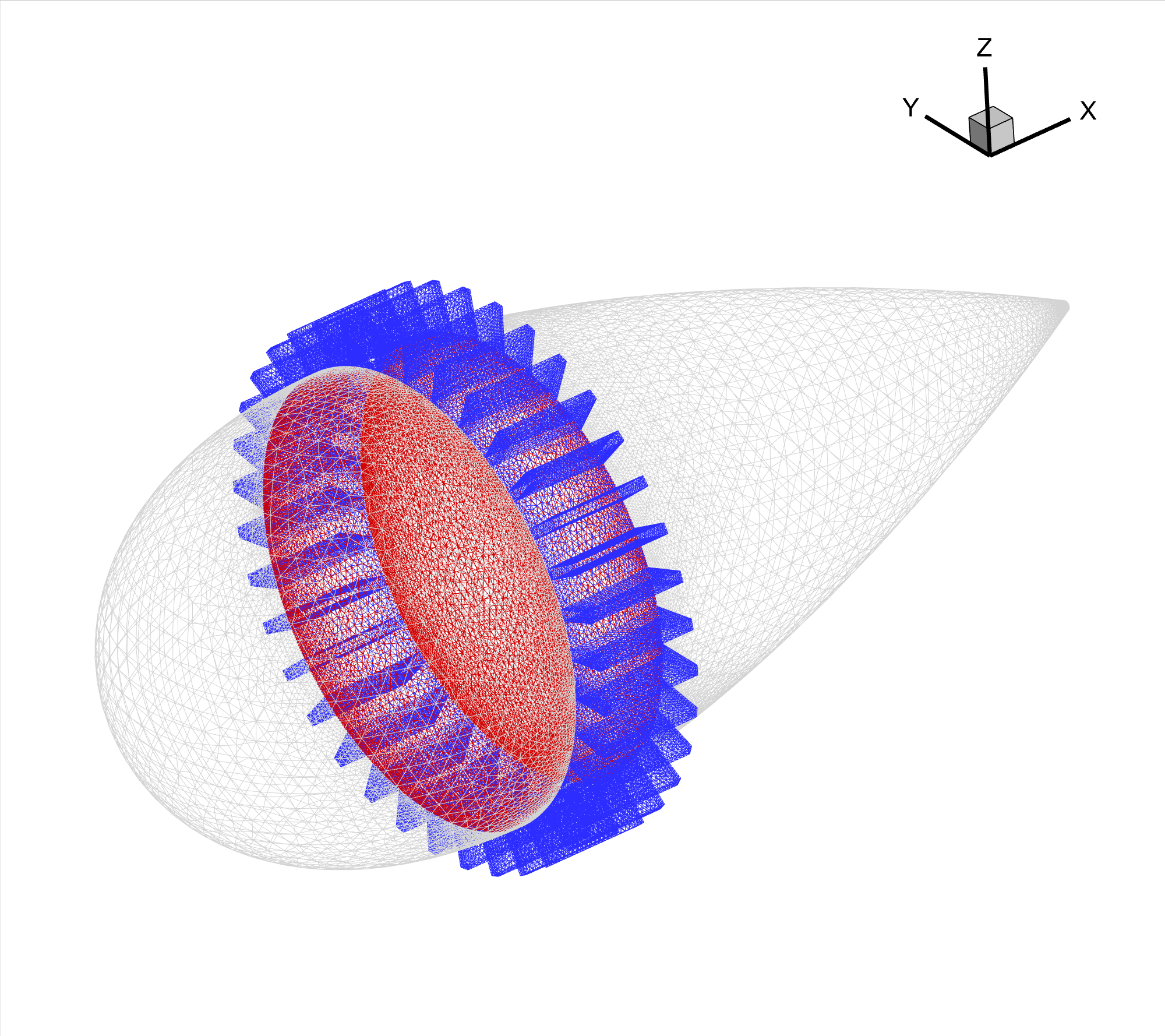
Fig. 7.8.1 Surface mesh. The gray, blue and red colors correspond to the centerbody, interface and adiabatic boundary conditions.

As shown in Fig. 7.8.2, when generating the volume mesh, we need to create two blocks: solid (red) and fluid (blue). All cells inside the solid block are required to be tetrahedral elements. Additionally, the cells on the interface need to match, so the interface cells need to be triangular.

Fig. 7.8.2 Volume mesh. Left: sliced at Y = 0 m. Right: sliced at X = 0.35 m

The mesh file for this tutorial is provided so that you can easily replicate this example in your own account.

7.8.2. Case

In this section, we will guide you on how to prepare the Flow360.json file. Let’s start by specifying the freestream conditions, which are listed below:

• Density \(\rho_\infty = 1.225 \ \text{kg}/\text{m}^3\)

• Speed of sound \(C_{\infty} = 340 \ \text{m/s}\)

• Temperature \(T_\infty = 288.15 \ \text{K}\)

• Mach \(= 0.1\)

Additionally, it is important to note that the grid unit used in this example is 1 meter, denoted as \(L_\text{gridUnit} = 1 \ \text{m}\).

7.8.2.1. boundaries

The boundaries subsection in Flow360.json is shown as follows:

"boundaries": {
   "fluid/farfield": {
      "type": "Freestream"
   },
   "fluid/centerbody": {
      "type": "NoSlipWall"
   },
   "solid/adiabatic": {
      "type": "SolidAdiabaticWall"
   }
}

7.8.2.2. volumeZones

The material of the solid part is copper, and the thermal conductivity for copper is \(k = 398 \ \text{W}/(\text{m} \cdot \text{K})\). The reference thermal conductivity for nondimensionalization is given by,

(7.8.1)\[k_\text{ref} = \frac{\rho_{\infty} C_{\infty}^3 L_\text{gridUnit}}{T_{\infty}} \approx 167091 \ \text{kg}/(\text{s}^3 \cdot \text{m})\]

Therefore, the nondimensional thermalConductivity can be written as:

(7.8.2)\[\text{thermalConductivity} = \frac{k}{k_\text{ref}} \approx 0.00238\]

Consider a heat source uniformly distributed in the solid block. The power of the heat source is \(5 \ \text{kW}\), the volume of the cylindrical solid is roughly \(\pi R^2 L \approx 0.01257 \ \text{m}^3\). So the volumetric heat source \(\dot{q}\) can be written as:

(7.8.3)\[\dot{q} = \frac{5 \ \text{kW}}{0.01257 \ \text{m}^3} \approx 398 \ \text{kW}/\text{m}^3\]

The reference volumetric heat source for nondimensionalization is given by,

(7.8.4)\[\dot{q}_\text{ref} = \frac{\rho_\infty C_\infty^3}{L_\text{girdUnit}} = 48147400 \ \text{kg}/(\text{s}^3 \cdot \text{m}) \approx 48147 \ \text{kW}/\text{m}^3\]

Therefore, the nondimensional volumetric heat source is,

(7.8.5)\[\text{volumetricHeatSource} = \frac{\dot{q}_s}{\dot{q}_\text{ref}} \approx 0.00826\]

For more details regarding the nondimensionalization of thermalConductivity and volumetricHeatSource, please see nondimensional inputs in the knowledge base.

The volumeZones subsection in Flow360.json is shown as follows,

"volumeZones": {
   "fluid": {
      "modelType": "FluidDynamics"
   },
   "solid": {
      "modelType": "HeatTransfer",
      "thermalConductivity": 0.00238,
      "volumetricHeatSource": "0.00826"
   }
},

Note that volumetricHeatSource is a string. For a nonuniform heat source, it could be an expression that contains variables x, y and z. For more details about the volumeZones subsection, see volumeZones in the solver configuration page.

7.8.2.3. heatEquationSolver

In addition to the navierStokesSolver and turbulenceModelSolver, a new subsection heatEquationSolver is also needed to control the convergence of the CHT solver. As shown in the following example, for steady-state simulations, there are two absoluteTolerance:

1. Outer absoluteTolerance: This is the overall convergence criterion for the steady-state simulation. If the absolute residual drops below this value, then the simulation is allowed to stop before reaching the maxPseudoSteps.

2. Inner absoluteTolerance: This is the local convergence criterion within each pseudostep. When running the linear solver, if the absolute residual drops below this value, then the heat solver will skip to the next pseudostep.

"heatEquationSolver": {
   "absoluteTolerance": 1e-11,
   "linearSolverConfig": {
      "maxIterations": 25,
      "absoluteTolerance": 1e-12
   },
   "equationEvalFrequency": 10,
},

More details about the heatEquationSolver can be found in heatEquationSolver in the solver configuration page. For your convenience, the complete Flow360.json is also provided here.

7.8.3. Results

The temperature fields directly outputted by Flow360, labeled as T, are nondimensional. To convert these nondimensional temperatures back to physical temperatures in Kelvin, you need to multiply them by the reference temperature \(T_\infty = 288.15 \ \text{K}\). The physical temperature distribution on the surface and solid domain are shown in Fig. 7.8.3 and Fig. 7.8.4.

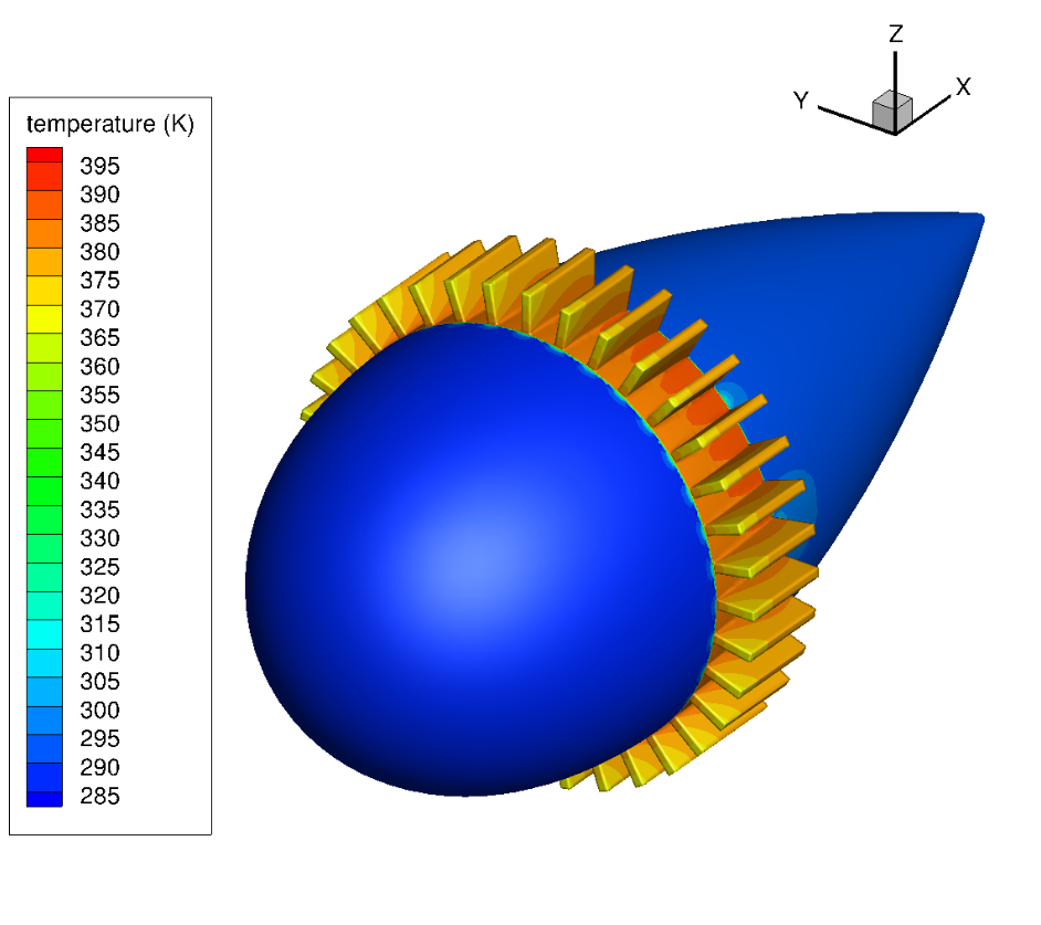
Fig. 7.8.3 Temperature field on the surface

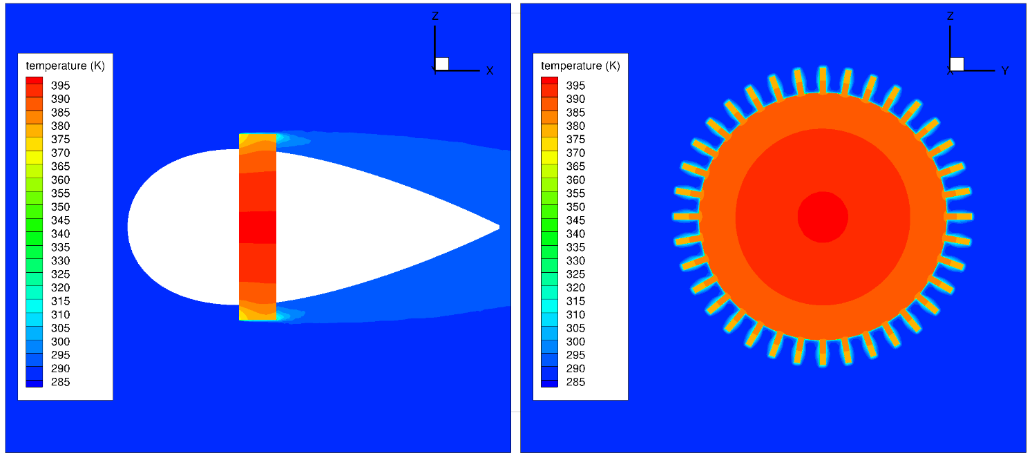
Fig. 7.8.4 Temperature field. Left: sliced at Y = 0 m. Right: sliced at X = 0.35 m.

Please note that the reference temperature \(T_\infty = 288.15 \ \text{K}\) provided here is for illustrative purposes, and you should adjust it according to the specific reference temperature used in your simulation.