RANS CFD on 2D High-Lift System Configuration Using the Flow360 Python API
Contents
6.2. RANS CFD on 2D High-Lift System Configuration Using the Flow360 Python API#
In this tutorial, we will look at a 2D multi-element airfoil which consists of a slat, wing, and flap. We will demonstrate how to create a general multi-element configuration model in ESP and
use the Flow360 Python API to run a RANS simulation. On this page you will find step-by-step instructions on how to:
Build a general quasi-3D multi-element configuration model in ESP
Set up automatic meshing and execute a RANS simulation
Use the Flow360 Python API to automatically update the configuration and re-submit a case
Firstly, we will explain how to build a general multi-element configuration model in Engineering Sketch Pad (ESP) and how to use edge, face, and group attributes to prepare that model for automatic meshing.
Then we will use that general model to build three standard test cases. The first case is a 3-element airfoil that is a cross-section of the NASA CRM-HL configuration and is used in a special session at AIAA Aviation 2020 called Mesh Effects for CFD Solutions.
There is no experimental data for this case and we only compare CFD results. The second case is 30P30N High-Lift Configuration, for which we have experimental data to compare to. The third case is the GA(W)-2 airfoil with a 30% fowler flap for which we also have experimental data.
Finally, we will set up the automatic meshing input files and use the Flow360 Python API to run a RANS simulation. The results of these simulations will then be validated against computational and experimental data.
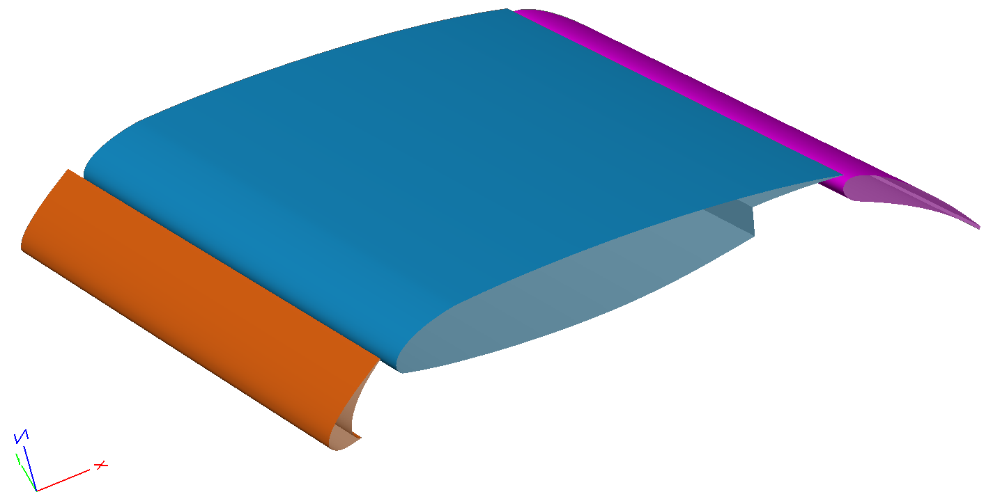
Fig. 6.2.1 quasi-3D high-lift system configuration generated in ESP#
Note
In this tutorial, we demonstrate how to build a quasi-3D model for a general high-lift system configuration in ESP.
The quasi-3D model here means extrusion of the 2D configuration.
ESP uses the OpenCSM (Open-source Constructive Solid Modeller) system which is a feature-based, associative, parametric solid modeler.
More information about ESP installation is available here. To build the geometry through ESP, we use a series of statements and commands in a script.
All ESP statements and commands are held in a *.csm file.
In this tutorial, we follow a “bottom-up” approach to build a general model for a multi-element configuration including wing, flap and slat.
To build the model, we start by defining the design, configuration and constant parameters.
The design parameter in this tutorial is the flap deflection angle. To define a design parameter, we use DESPMTR.
Design parameters describe any particular instance of the geometry model. They can be single-valued, 1D vectors, or 2D arrays of numbers.
Each design value has a current value, upper- and lower-bounds. ESP allows to compute the sensitivity of any part of a geometry model with respect to
any design parameter.
DESPMTR $pmtrName values
use: define a design Parameter
For the multi-element configuration, we also need to define the flap deflection axis location as a configuration parameter.
Since this is a quasi-3D model, the span of the quasi-3D model is also a configuration parameter.
To define a configuration parameter, we use CFGPMTR.
Values for the configuration parameters are declared in the top-level include-type .udc file. They must contain one or more numbers.
They must be dimension-ed, in case they are multi-valued. They have lower- and upper-bounds. Their values can be changed and sensitivities
cannot be computed for them.
CFGPMTR $pmtrName value
use: define a configuration Parameter
To build a general model for the multi-element configuration, we need to consider that we may not have flaps, or slats or either.
Therefore, their presence in configuration parameters can be defined as a constant parameter for each. To define a constant parameter in a build process, we use CONPMTR.
Constant parameters contain only one number. Their values are declared in the top-level include-type .udc file and are visible from any .csm or .udc file.
Their values cannot be changed and sensitivities cannot be computed for constant parameters.
CONPMTR $pmtrName values
use: define a constant Parameter
The example below shows how to put these statements all together in a CSM file.
In this example, DIMENSION indicates the size of the array used to define the flap deflection axis location.
DIMENSION $pmtrName nrow ncol
use: set up or redimensions an array Parameter
The flap deflection angle is defined in degrees. The span is in meters. The status parameter for the flap and slat indicates if they are present in the configuration.
Any value other than zero indicates that they are present in the configuration.
In this section, we define a wire body for each element in the configuration. Then, we create a face (e.g. a higher type) from that wire body.
This section is similar to creating 3D sketches for airfoils in the ONERA M6 Wing Geometry Modeling.
To create a sketch body for each element, we use the following format:
The above CSM example shows how to put together a 3D sketch for an airfoil. These 3D sketches are later used to build a face body and then face bodies are used to be extruded into a solid body.
In this example, we follow a simple concept to define a 2D curve. We define all the curves directly in global 3D space. In case, we need them on a plane, we define 3D data as needed.
For example, we define the multi-element configuration on the xz-plane. Therefore, we create all splines in the global 3D space by setting all y-coordinates of the 3D points to zero.
As shown in the above example, all 3D sketches start from the upper trailing-edge point to the leading-edge point and back to the lower trailing-edge point. This means the points definition is counter-clockwise.
In a multi-element configuration, we have three elements including the wing, which is the main element, the slat in front of the wing, and the flap in the back. The wing element profiles can have two curves defined through
two splines, when there is a concave region in the back where the flap closes in. It can have more curves when the flap element is present. Since we define a generic multi-element modeler, we include all possible situations.
Therefore, wing element profiles always include two curves defined by two splines connected at the leading-edge. If the flap element is present in the configuration,
we define a curve using a single spline in a separate sketch for the concave region in the back of the wing.
For the flap element, we have two curves defined by two splines in one sketch. For the slat element, we have two curves: the front and back curves. The front curve is defined with two spline in one sketch.
The back curve is defined with one spline in a different sketch.
Please note that when we define a single spline in a sketch, we don’t need to group it.
Here you can find the complete CSM file for this step including the sketches for three elements in the configuration: multielementStep2.csm.
In this section, we restore the sketch body for each element and create a face from them.
RESTORE $name index=0
use: restores Body(s) that was/were previously stored
In the above description, “=” indicates an optional argument for the statement. When the optional argument is not indicated, the default value after the equal sign is taken.
To create a face body from a wire body, we use combine.
COMBINE toler=0
use: combine Bodys since Mark into next higher type
In this tutorial, we close the wire body and then use join to have one single wire body before calling the combine statement.
JOIN toler=0 toMark=0
use: join two Bodys at a common Edge or Face
Because we create a general model for multi-element configuration, to close a wire body for each element, we have different scenarios.
Two possible scenarios to create a closed wire body for the wing element are explained below.
Note
Wing Element Scenario A:
The flap status is not equal to 1, which means there is no flap element in the configuration. Therefore, the wing wire body only includes the upper and the lower curves forming
an airfoil. To close the wire body, we can connect the upper and the lower trailing-edge points with a line sketch.
Wing Element Scenario B:
The flap status is equal to 1, which means there is a flap element in the configuration. Therefore, the wing wire body includes three spline curves forming the
upper wing, the lower wing and the concave curve in the rear portion of the wing. Based on the format explained in the 3D Sketch Format:
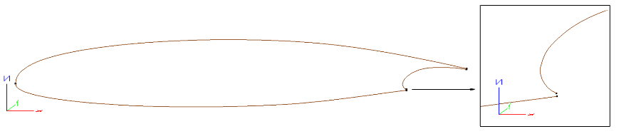
The concave curve starts from the lower trailing-edge point and it ends up connected to the lower curve of the wing. In the figure below, as an example, the wing element for the 2D CRM high-lift configuration is shown. In this configuration, we have a flap element and the concave curve in the back of the wing is connected to the lower curve of the wing element, which creates a sharp point in the connection.
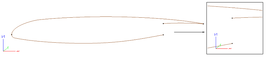
The concave curve starts from the lower trailing-edge point and it does not end up connected to the wing lower curve. In the figure below, as an example, the wing element for the 30p30n high-lift configuration is shown. In this configuration, we have a flap element and as you see, the concave line in the back of the wing element is not connected to the lower curve of the wing. To create a closed wire body for the wing element, we need to connect the ending point of the concave curve to the ending point of the lower curve of the wing element.
In the figure below, the wing element for the GA(W)-2 high-lift configuration is shown. As you see, we have a flap element in this configuration and the concave curve in the back of the wing is not connected to
the lower curve of the wing. To create a close wire-body, we have to connect the ending point of the concave curve to the ending point of the lower curve of the wing. This is the second item in scenario B and it creates a blunt trailing-edge in the connection.
To cover both types of curves in the concave rear part of the wing, first we connect the upper trailing-edge point to the
lower trailing-edge point and then in case the concave curve is not connected to the wing lower curve, we use a line sketch to connect it and close
the wire body for the wing.
Based on the above-mentioned scenarios, first we restore the wing sketch group and join it. Therefore, we have one wire body including
two edges and three nodes.
restore wing
join
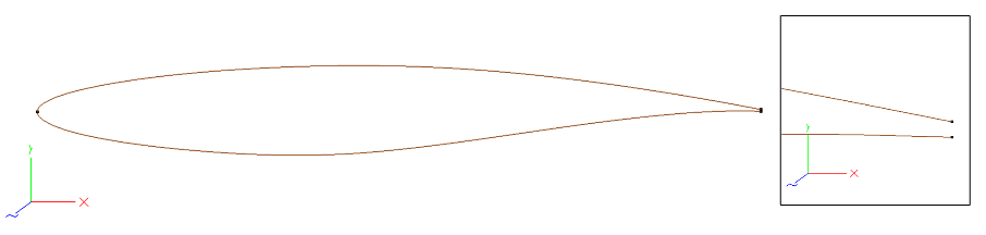
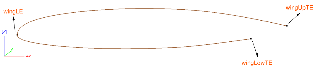
Then, we must find the coordinates of these three nodes representing the leading-edge and the upper and lower trailing-edge. To find their coordinates, we loop over all the nodes in the
current body and detect the leading-edge node and the trailing-edge nodes based on their x and z values. The leading-edge node and the trailing-edge nodes for a wing wire with flap is shown below.
Fig. 6.2.2 Leading-edge and trailing-edge nodes for a wing profile#
# defining arrays with one row and three columnsdimensionwingLE13dimensionwingUpTE13dimensionwingLowTE13# initializing xmin, zmin, zmax with their opposite extremessetxmin@xmax
setzmin@zmax
setzmax@zmin
# looping over nodes to find the LEsetnNodes@nnode
patbeginodenNodes
evaluatenode@ibodyinode
IFTHEN@edata[1]LTxmin
setxmin@edata[1]setwingLE"xmin;@edata[2];@edata[3];"setleadingNodeIDinode
ENDIFpatend# looping over nodes to find the TEpatbeginodenNodes
IFTHENinodeNEleadingNodeID
evaluatenode@ibodyinode
IFTHEN@edata[3]GTzmax
setzmax@edata[3]setwingUpTE"@edata[1];@edata[2];zmax;"ENDIFIFTHEN@edata[3]LTzmin
setzmin@edata[3]setwingLowTE"@edata[1];@edata[2];zmin;"ENDIFENDIFpatend
Note
In this tutorial, a “bottom up” approach is provided. The solid body is built up from nodes, to curves, to edges, to surfaces, to faces, to shells, and finally bodies.
The term ‘node’ here refers to the nodes at the ends of each edge, which differs from the airfoil data points used to define the upper and lower curves.
In the above code, first we define arrays for the leading-edge and trailing-edge nodes.
Then we assign the maximum value of the x-axis in this current body as the initial value for the xmin variable,
the maximum value of the z-axis in this current body as the initial value for the zmin variable, and the minimum value of the
z-axis in this current body as the initial value for the zmax variable.
Then we collect the total number of nodes in this current body by using node, loop over them, evaluate them, and compare
the x value of their coordinates with the xmin to find the leading-edge node. When x coordinate of a node has a value less than xmin,
the value of xmin is updated with that x value. We also store the nodeID at each update in the leadingNodeID.
In this case, the leading-edge node is the most forward one, hence with the lowest x coordinate. Each wire body is composed of only edges and each edge has two nodes including the begin and end nodes.
When we collect all the nodes in the current body, we collect all the ending nodes for all of the edges. Please note the node here refers to the node as one of the topological entities and it is different
from the airfoil data points used to create the spline.
Then we loop over all nodes again and if the nodeID is not equal to leadingNodeID, we evaluate and compare the value of z coordinate to
find the upper trailing-edge node with maximum z and the lower trailing-edge node with minimum z. The way we find the leading-edge and trailing-edge nodes in this example is similar to adding edge attributes based on node coordinates in the ONERA M6 Wing Geometry Modeling.
For a detailed description you can refer to that tutorial.
After restoring the wing wire body, we restore the sketch spline for the concave line in the rear of the wing, if the flap status is not equal to zero.
Just like we did for the upper and lower curves above, we will now find the begin and end points of the concave spline.
Therefore, after we restore the concave spline sketch, we define two arrays for the coordinates of the starting and ending points, then we
initialize the xmin and xmax variables with the maximum and minimum x values of the current sketch body.
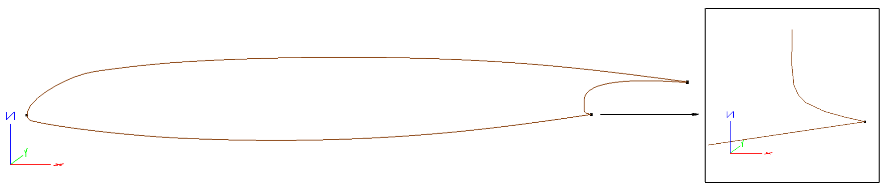
To find the starting point, which has minimum x value, and the ending point, which has the maximum x value, we loop over all the nodes and evaluate the coordinates
of each node. If the value for the x coordinate were less than the xmin variable, we update the xmin variable. We follow the same technique to find then ending point
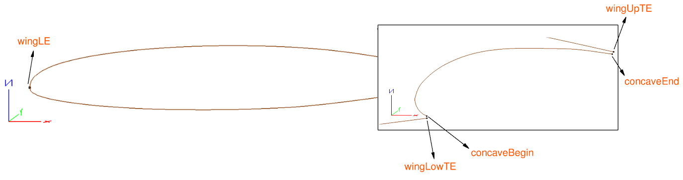
with the xmax variable. The ending nodes of the concave spline is shown below in comparison to ending nodes of the wing profile.
Fig. 6.2.3 Ending nodes of the concave spline for a wing profile.#
patbegthenifzero(flapStatus,0,1)# restoring sketchrestorewingConcave
# defining arrays for the ending nodesdimensionconcaveEnd13dimensionconcaveBegin13# initializing xmin and xmax with their opposite extremessetxmax@xmin
setxmin@xmax
# looping over nodes to find the ending pointspatbeginode@nnode
evaluatenode@ibodyinode
IFTHEN@edata[1]GTxmax
setxmax@edata[1]setconcaveEnd"xmax;@edata[2];@edata[3];"ENDIFIFTHEN@edata[1]LTxmin
setxmin@edata[1]setconcaveBegin"xmin;@edata[2];@edata[3];"ENDIFpatend# connecting the wing upper TE node to the ending node of the wing concave curve with line segmentskbegconcaveEnd[1]concaveEnd[2]concaveEnd[3]linsegwingUpTE[1]wingUpTE[2]wingUpTE[3]skend# calculating the distance between the wing lower TE node and starting node of the wing concave linesetsum0patbegi3setsumsum+(concaveBegin[i]-wingLowTE[i])^2patendsetdistancesqrt(sum)IFTHENdistanceGT1e-04
# connecting the wing lower TE node to the starting node of the wing concave curve with line segmentskbegconcaveBegin[1]concaveBegin[2]concaveBegin[3]linsegwingLowTE[1]wingLowTE[2]wingLowTE[3]skendENDIFpatend
After we have obtained the starting and ending point of the concave spline sketch, we connect the upper trailing-edge point of the wing to the ending node of the
concave curve with a sketch and a line segment. Then we need to find out if the concave spline sketch is connected to the lower trailing-edge node of the wing spline sketch or not.
For that purpose, we calculate the distance between two nodes: the lower trailing-edge node of the wing spline sketch and the starting node of the concave spline sketch.
When this distance is zero, these two splines sketches are connected and share the same node; otherwise we define a sketch and use a line segment to connect them and close
the wire body.
Finally we use combine to elevate the wire body into a face, and then store it as a face.
After we built the wing face, we check the flap and slat status. If they are set to be present in the configuration, we build their faces.
patbegthenifzero(flapStatus,0,1)restoreflap
join# defining arrays for the leading-edge and trailing-edge nodesdimensionflapLE13dimensionflapUpTE13dimensionflapLowTE13# initializing xmin, zmin and zmax with their opposite extremessetxmin@xmax
setzmin@zmax
setzmax@zmin
# looping over nodes to find the leading-edge nodesetnNodes@nnode
patbeginodenNodes
evaluatenode@ibodyinode
IFTHEN@edata[1]LTxmin
setxmin@edata[1]setflapLE"xmin;@edata[2];@edata[3];"setleadingNodeIDinode
ENDIFpatend# looping over nodes to find the trailing-edge nodespatbeginodenNodes
IFTHENinodeNEleadingNodeID
evaluatenode@ibodyinode
IFTHEN@edata[3]GTzmax
setzmax@edata[3]setflapUpTE"@edata[1];@edata[2];zmax;"ENDIFIFTHEN@edata[3]LTzmin
setzmin@edata[3]setflapLowTE"@edata[1];@edata[2];zmin;"ENDIFENDIFpatend# closing the flap wire body by a line segmentskbegflapLowTE[1]flapLowTE[2]flapLowTE[3]linsegflapUpTE[1]flapUpTE[2]flapUpTE[3]skend# creating a face body from the wire bodycombinestoreflapFace
patend
Like the wing face example, after we restore the flap sketch group, we use join to have a single wire body.
Then, we use dimension to define arrays for the coordinates of the leading-edge and trailing-edge nodes. The we initialize xmin, zmin and zmax
variables for the nodes in the flap wire body with the maximum value of x, maximum value of z and minimum value of z for the current body.
Then we loop over all the nodes, evaluate at each node, and compare the x value of the node to find the leading-edge node. We use the same technique
to find the trailing-edge nodes. Then, we close the flap wire body with a line segment and finally elevate the wire body to the face and store it.
For the slat wire body, we follow the same approach. In comparison to the flap, the only difference is that the slat has two-spline sketches forming the front curve and one spline sketch in the back.
patbegthenifzero(slatStatus,0,1)# restore the front spline sketchrestoreslatFront
join# defining arrays for the leading-edge and trailing-edge nodesdimensionslatFrontLE131dimensionslatFrontUpTE131dimensionslatFrontLowTE131# initializing xmin, zmin and zmax with their opposite extremessetxmin@xmax
setzmin@zmax
setzmax@zmin
# looping over nodes to find the leading-edge nodesetnNodes@nnode
patbeginodenNodes
evaluatenode@ibodyinode
IFTHEN@edata[1]LTxmin
setxmin@edata
setslatFrontLE"xmin;@edata[2];@edata[3];"setleadingNodeIDinode
ENDIFpatendpatbeginodenNodes
IFTHENinodeNEleadingNodeID
evaluatenode@ibodyinode
IFTHEN@edata[3]GTzmax
setzmax@edata[3]setslatFrontUpTE"@edata[1];@edata[2];zmax;"ENDIFIFTHEN@edata[3]LTzmin
setzmin@edata[3]setslatFrontLowTE"@edata[1];@edata[2];zmin;"ENDIFENDIFpatend# restore the back spline sketchrestoreslatBack
# defining arrays for the trailing-edge nodesdimensionslatBackUpTE131dimensionslatBackLowTE131# initializing xmin, zmin and zmax with their opposite extremessetzmin@zmax
setzmax@zmin
# looping over nodes to find the trailing-edge nodessetnNodes@nnode
patbeginodenNodes
evaluatenode@ibodyinode
IFTHEN@edata[3]GTzmax
setzmax@edata[3]setslatBackUpTE"@edata[1];@edata[2];zmax;"ENDIFIFTHEN@edata[3]LTzmin
setzmin@edata[3]setslatBackLowTE"@edata[1];@edata[2];zmin;"ENDIFpatend# closing the trailing edge at the bottom side of the slatskbegslatFrontLowTE[1]slatFrontLowTE[2]slatFrontLowTE[3]linsegslatBackLowTE[1]slatBackLowTE[2]slatBackLowTE[3]skend# closing the trailing edge at the top side of the slatskbegslatFrontUpTE[1]slatFrontUpTE[2]slatFrontUpTE[3]linsegslatBackUpTE[1]slatBackUpTE[2]slatBackUpTE[3]skend# creating a face body from the wire bodycombinestoreslatFace
patend
For the slat element, we have two edges defining the front curve and connected at the leading-edge, and one edge in the back.
In the above code, we use the same technique we used for the wing and flap elements to find the leading-edge and trailing-edge nodes for the slat element.
After that, we restore the slat’s back spline sketch. It is a single spline; therefore we don’t need to join.
Then, we define two arrays to find the upper and the lower nodes, initialize zmin and zmax variables, and loop over the nodes to find the upper and the lower nodes.
At the end, we use a line segment sketch to connect the trailing-edge nodes at the top of the slat and at the bottom side of the slat.
Now that the wire body is closed, we use combine to elevate the wire body into a face body.
In this section, we build the solid body for the each element from their face bodies.
# restoring faces to build solid body | wingrestorewingFace
extrude0span0storewingBody
# restoring faces to build solid body | flappatbegthenifzero(flapStatus,0,1)restoreflapFace
extrude0span0rotateyflapDeflectionflapDefAxis[3]flapDefAxis[1]storeflapBody
patend# restoring faces to build solid body | slatpatbegthenifzero(slatStatus,0,1)restoreslatFace
extrude0span0storeslatBody
patend
In the above code, for each element we restore their face and then we use the extrude statement to build the solid body.
After the extrusion, we store the body. The span parameter is defined in the preamble.
EXTRUDE dx dy dz
use: create a Body by extruding an Xsect
Since we are building a generic model for a multi-element configuration and we have defined a flap deflection angle as a design parameter, after extruding the flap face body, we rotate the
flap solid body around the flap deflection axis by using the rotatey statement.
ROTATEY angDeg zaxis=0 xaxis=0
use: rotates Group on top of Stack around an axis that passes through (xaxis, 0, zaxis) and is parallel to the y-axis
After building the solid models for the multi-element configuration, we must add edge attributes to each element and prepare them for automatic meshing.
To add the edge attribute, we use the node coordinates that were obtained above when we elevated the wire body into a face body.
To add edge attributes, we use EdgeAttr udprim. This udprim is shipped with the pre-built version of the ESP on Flexcompute’s GitHub page.
We add edge attributes for each element after the extrusion and before the restore. For example for the wing element, we have two
symmetric edges, one leading-edge and two trailing-edges.
# restoring faces to build solid body | wingrestorewingFace
extrude0span0# adding edge attributes | wingdimensionySymm21setySymm"0;span;"patbegi2udpargedgeAttrattrname$edgeNameattrstr$symmetryudprimedgeAttrxyzs"wingLE[1];ySymm[i];wingLE[3];wingUpTE[1];ySymm[i];wingUpTE[3];"udpargedgeAttrattrname$edgeNameattrstr$symmetryudprimedgeAttrxyzs"wingLE[1];ySymm[i];wingLE[3];wingLowTE[1];ySymm[i];wingLowTE[3];"patbegthenifzero(flapStatus,0,1)udpargedgeAttrattrname$edgeNameattrstr$symmetryudprimedgeAttrxyzs"concaveBegin[1];ySymm[i];concaveBegin[3];concaveEnd[1];ySymm[i];concaveEnd[3];"udpargedgeAttrattrname$edgeNameattrstr$symmetryudprimedgeAttrxyzs"wingUpTE[1];ySymm[i];wingUpTE[3];concaveEnd[1];ySymm[i];concaveEnd[3];"IFTHENdistanceGT1e-04
udpargedgeAttrattrname$edgeNameattrstr$symmetryudprimedgeAttrxyzs"concaveBegin[1];ySymm[i];concaveBegin[3];wingLowTE[1];ySymm[i];wingLowTE[3];"ENDIFpatendpatendudpargedgeAttrattrname$edgeNameattrstr$wingleadingEdgeudprimedgeAttrxyzs"wingLE[1];wingLE[2];wingLE[3];wingLE[1];span;wingLE[3];"udpargedgeAttrattrname$edgeNameattrstr$wingtrailingEdgeudprimedgeAttrxyzs"wingUpTE[1];wingUpTE[2];wingUpTE[3];wingUpTE[1];span;wingUpTE[3];"udpargedgeAttrattrname$edgeNameattrstr$wingtrailingEdgeudprimedgeAttrxyzs"wingLowTE[1];wingLowTE[2];wingLowTE[3];wingLowTE[1];span;wingLowTE[3];"patbegthenifzero(flapStatus,0,1)udpargedgeAttrattrname$edgeNameattrstr$wingtrailingEdgeudprimedgeAttrxyzs"concaveEnd[1];concaveEnd[2];concaveEnd[3];concaveEnd[1];span;concaveEnd[3];"udpargedgeAttrattrname$edgeNameattrstr$wingtrailingEdgeudprimedgeAttrxyzs"concaveBegin[1];concaveBegin[2];concaveBegin[3];concaveBegin[1];span;concaveBegin[3];"patendstorewingBody
For the wing element, we have three types of edges including: leading-edge, trailing-edge and symmetric.
We consider edges associated with the concave region of the multi-element configuration as trailing-edges when the flap status is nonzero.
Therefore, in the above code, we define an array with two elements including zero and span. These two elements define two symmetric planes for the
multi-element configuration quasi-3D model. For the symmetric edges, we call the edgeAttr udprim twice. When the flap status is nonzero,
we must also add the edge attribute for edges associated with the concave region. In the Building the Wing Face Body, we
defined and calculated a distance parameter to find out if the concave spline was connected to the wing lower trailing-edge node.
We use the same parameter here to add the edge attributes to associated edges in the concave rear part. This is for when the wing lower trailing-edge node is not
connected to the starting node of the concave sketch spline.
For the leading-edge, we use the wingLE array defined in the above sections to add the edge attribute. For the trailing-edge, we use wingUpTE and wingLowTE arrays to
add the edge attributes. When the flap status is nonzero, we use concaveBegin and concaveEnd arrays to add edge attributes to concave spanwise lines
associated with the rear concave region of the wing element.
For the flap and slat elements, we follow the same procedure to add edge attributes to the leading-edge and trailing-edge.
After we added the edge attributes for each element, we must add the face and group attributes and prepare the model for the automatic meshing.
# restoring bodies to add face and group attributes | wingrestorewingBody
# adding face and group attributes to the entire solid bodyattributefaceName$wingattributegroupName$wingsetnWingFaces@nface
setsumWingArea@area
setminAreasumWingArea
# finding the face with min are | wing trailing edge facepatbeginWingFaces
selectfacei
IFTHEN@areaLTminArea
setminArea@area
settrailingFaceIDi
ENDIFpatend# adding face and group attributes to the wing trailing faceselectfacetrailingFaceID
attributefaceName$wingTrailingattributegroupName$wing
In the above example, we restore the wing solid body and then we use attribute statement to add a string value ‘wing’ to the
attribute name faceName and to add the same string value to the attribute name ‘groupName’. The statement attribute is defined below.
When the first letter of the attribute value is a string, then it must be started with ‘$’.
ATTRIBUTE $attrName attrValue
use: sets an Attribute for the Group on top of Stack
After adding the ‘$wing’ as the attribute value to the attribute ‘faceName’ and ‘groupName’, we find the face with the minimum area and add ‘$wingTrailing’ as the
string value for the ‘faceName’ attribute. Like this, we can specify the maximum edge length for the surface mesh in the automatic meshing.
The ‘groupName’ attribute is same.
To find the face with the minimum area, we define a variable minArea and initialize it with the sum of all faces.
Then, we loop over all faces and compare their face area. When their face area is less than the value of the minArea, we update the minArea variable and
we store the faceID.
We follow the same procedure to add a string value to the ‘faceName’ and ‘groupName’ attributes.
Here you can find the complete CSM file for the multi-element configuration: multielementStep7.csm.
Using Python to Add Coordinates and Build Parameters#
So far, we have used ESP statements and written a script to build a general model for the multi-element configuration.
Now, we use a python script that lets us add the build parameters and data point coordinates for each element into the CSM script.
For this purpose, we divide the geometry modeling script with ESP statements into two parts: preamble and body. The preamble includes the build parameters
and the sketch splines. The body includes the rest of the build process: restore sketch bodies, build the solid model, and add attributes
to the solid body. Then, we save the body into a separate file and call it multielement.model.
The generateModel.py takes a JSON input file (ie, input_configuration.json) that holds the build parameters and path to the data point coordinates for each element.
Then, it adds them to the preamble of the multielement.model and saves the CSM file corresponding to the input JSON file. This CSM file later can be passed to ESP to build the model.
To execute the build process using the python script, make sure the generateModel.py and multielement.model are in the same directory, then run:
The “input_configuration.json” holds input build parameters and the configuration’s data coordinates.
These data coordinates define the concave line in the rear part of the wing, the wing, flap, and slat.
Each element’s data coordinates is defined in a separate file. For example, for the 2D CRM configuration, the input configuration JSON is:
The “this_configuration.csm” is the output of the generateModel.py. This file holds the build prescription for the configuration corresponding to the input configuration JSON file.
Users can later use it with ESP to build the complete model and check the build process.
When the slat and flap options are set to false in the input configuration JSON, only the quasi-3D model for the wing profile is created, which can be used to build a quasi-3D model for an airfoil.
All the associated files with this tutorial, including the input configuration JSON files, are available in multielement_tutorials.tar.gz. By executing the generateModel.py with different input configuration JSON files, you can build different multi-element models in ESP.
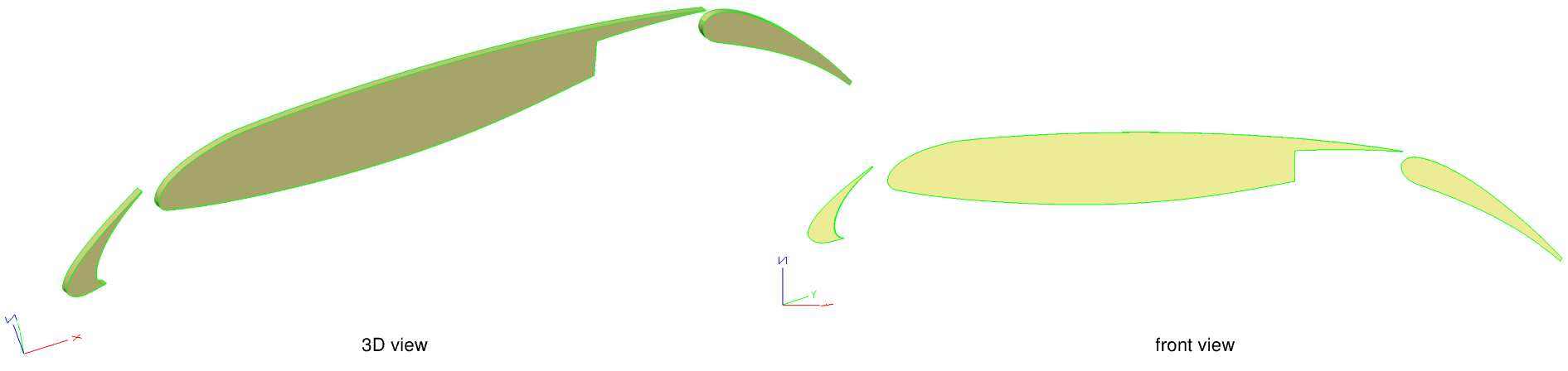
Below we can see the three standard test cases that will be used for the simulations.
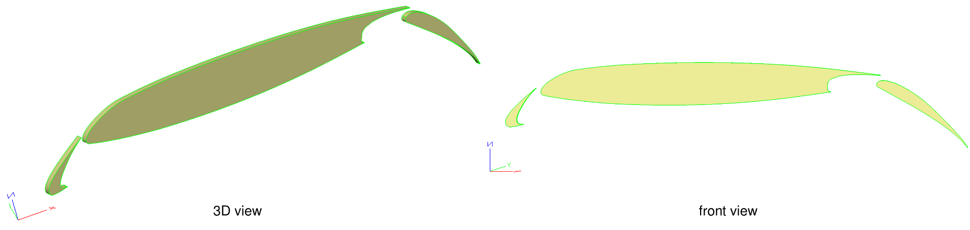
Fig. 6.2.4 Quasi-3D model generated in ESP 30p30n system configuration#
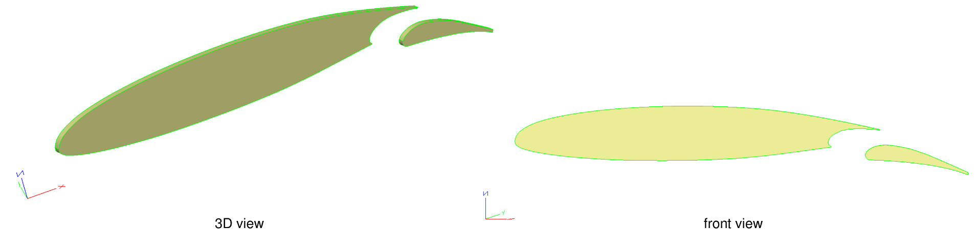
Fig. 6.2.5 Quasi-3D model generated in ESP for 2D CRM system configuration#
Fig. 6.2.6 Quasi-3D model generated in ESP GA(W)-2 system configuration#
RUN CFD on multi-element configurations using Flow360#
In this section, we show how to run CFD simulations using the Flow360 Python API for different multi-element configurations with different design parameters.
After using the generateModel.py to create the build prescription, we need to set up the input surface mesh JSON file and input volume mesh JSON file.
Then, we set up the case JSON and submit the simulation.
To control the mesh’s density in a particular region of the model, we use attributes defined in ESP. For a body, we have edge and face attributes.
The edge attribute indicates how to treat the surface mesh at that particular edge. The face attribute defines the maximum edge length for the unstructured surface mesh over that face.
In addition, for the entire surface mesh, there are three global parameters: surface_max_edge_length, curvature_resolution_angle, and
boundary_layer_growth_rate.
These parameters generate the surface mesh where edge and face attributes are not specified.
The curvature_resolution_angle defines how well the curved region of the model is captured by the unstructured mesh.
We use five cylindrical volume-mesh constraints for the volume mesh to let the unstructured mesh gradually grow out in the space surrounding the high-lift configuration.
For the volume mesh over the wall, we specify the initial height of the high-aspect-ratio anisotropic mesh and the growth ratio.
The Python script for setting up the meshing configuration of 2D CRM system is:
Now we will show you how to leverage the Flow360 Python API and ESP’s scripting capabilities to conduct a parametric design and simulation study for a general high-lift system configuration with three standard examples.
For any other multi-element configuration:
a. put data coordinate files in the “data” directory.
b. copy a configuration JSON file and modify it according to your configuration of interest.
c. generate the model by using the same python script:
The ‘2dCRMSim.json’, for example, here holds the path to the CSM, surface, and volume and Flow360 case JSON to submit the simulation.
For the 2D NASA 30p30n configuration:
$ python3runCase.py-json30p30nSim.json
For the 2D GA(W)-2 configuration:
$ python3runCase.py-jsongaw2Sim.json
For a customized case:
a. copy and modify the surface and volume JSON files according to your configuration.
b. copy and modify the Flow360 case JSON file for your simulation.
c. copy and modify the case JSON file according to the surface, volume and Flow360 case JSON files and run:
We use the Flow360 Python API client to download the surface and volume solutions for postprocessing purposes.
The downloadCase.py script downloads the solution files for the ‘caseId’ specified in the input JSON file.
The input JSON file has the following contents:
You will need to update it with the caseId alphanumeric string returned by the runCase.py call above.
To download the solutions, you can run the Python script:
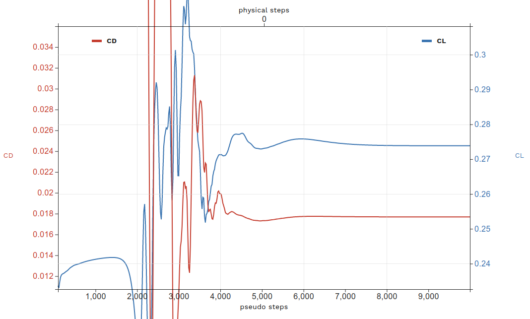
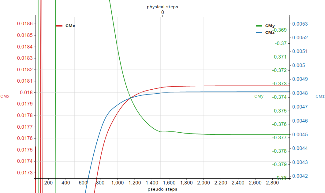
You can always find the convergence histogram on the Flow360 website, under your account, by clicking on your case name and selecting Convergence and Forces tabs.
For example, for the 2D CRM multi-element configuration, the convergence histories of forces are:
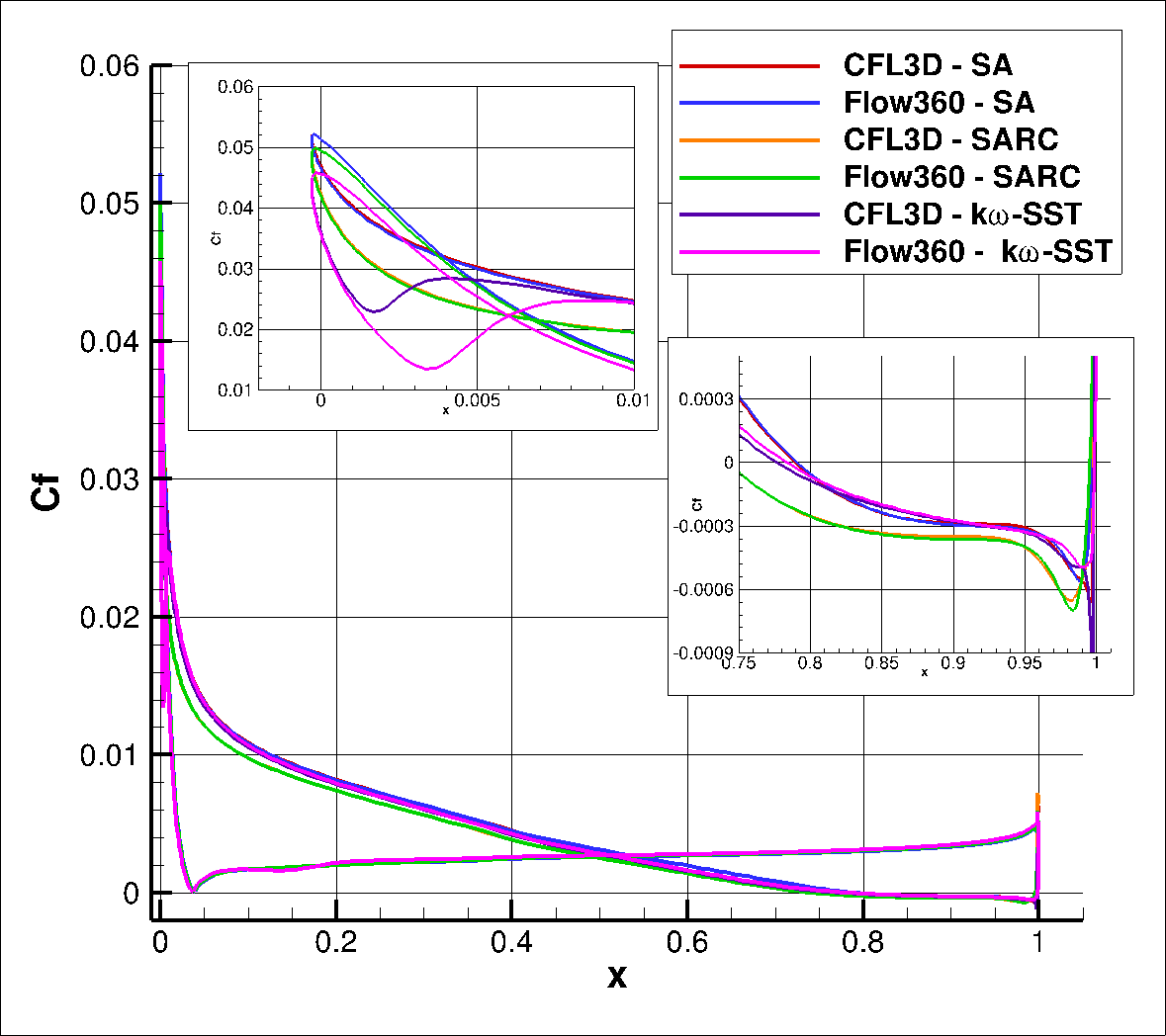
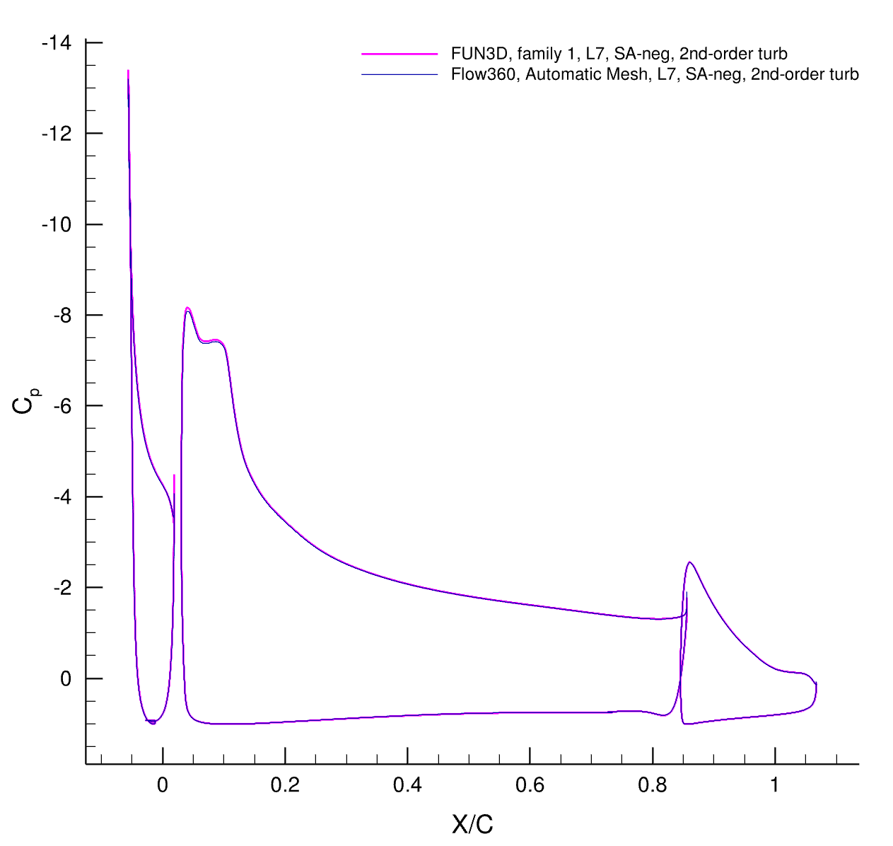
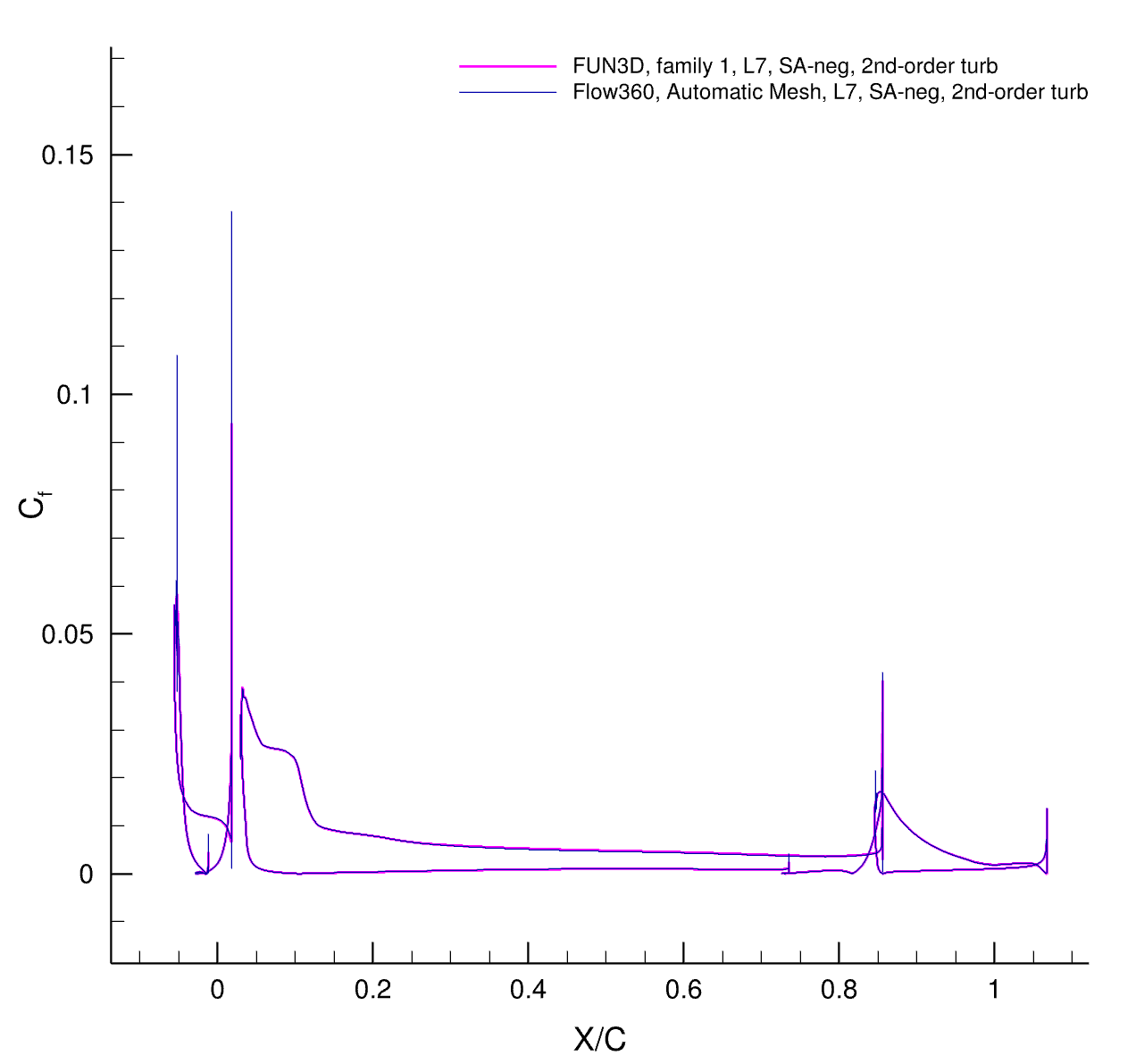
The surface pressure coefficient and skin friction coefficient from FUN3D on their finest grids are shown compared to Flow360 on the finest grid that is automatically generated using the Flow360 Python API.
The results agree well with each other.
Fig. 6.2.7 Surface pressure coefficient over the airfoil elements.#
Fig. 6.2.8 Skin friction coefficient over the airfoil elements.#
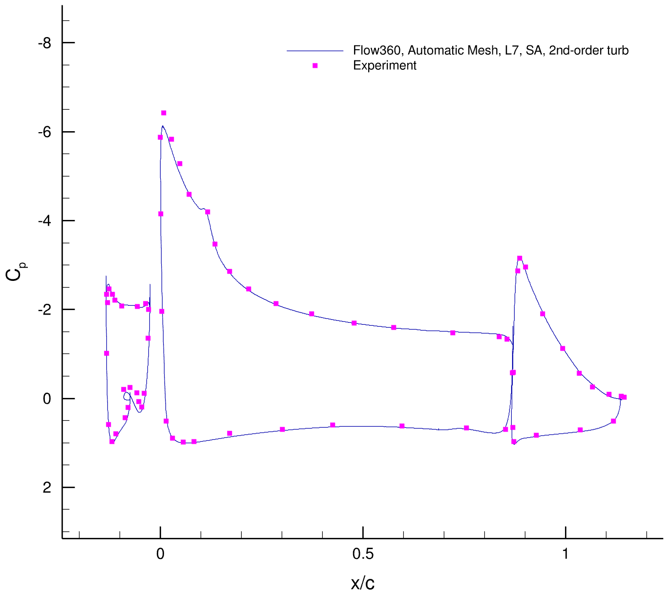
2D NASA 30p30n System Configuration:
The surface pressure coefficient and skin friction coefficient from FUN3D on their finest grids are compared to Flow360 on the finest grid, which is automatically generated using the Flow360 Python API.
The results agree well with each other.
Fig. 6.2.9 Surface pressure coefficient over the airfoil elements.#
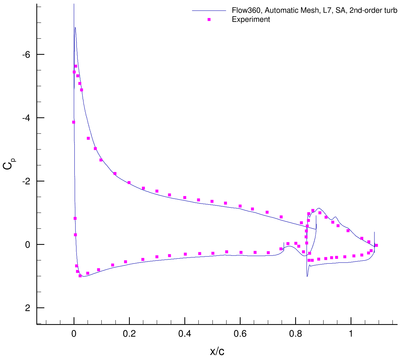
2D GA(W)-2 System Configuration with 30% Fowler Flap
Fig. 6.2.10 Surface pressure coefficient over the airfoil elements.#