6.8. TU Berlin TurboLab Stator simulation using periodic boundary conditions#
Description#
The “TurboLab Stator” is a stator enclosed in a measurement rig in the TU Berlin TurboLab. This geometry has been used in the past for CFD validation and optimization studies.
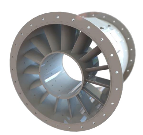
Fig. 6.8.1 TU Berlin TurboLab Stator#
This stator has 15 blades and because of its circular symmetry we can take advantage of the periodicity in the circumferential direction by simulating only 1 blade. This drastically reduces the meshing requirements and computing times. To do that we will use Periodic and Rotational to define rotationallyPeriodic boundary conditions. rotationallyPeriodic boundaries need to come in pairs, each is assigned the other as a match and the flow values of one are assigned to the other and vice versa. This ensures periodicity of the flow across those two boundaries.
rotationallyPeriodic boundaries are perfectly suited anytime the flow is axiperiodic and we can get away with simulating only a subset of the whole circular domain.
Note
This technique requires that both the flow conditions and geometry be axiperiodic. In this example, even though the geometry is axiperiodic, if the inflow had some alpha or beta value for example then this technique wouldn’t work. The same can be said if flow separation or unsteadiness makes the flow no longer axiperiodic.
Meshing the geometry#
When meshing a set of periodic boundaries it is important that both matched boundaries have the same shape and mesh topology so that the flow information from one boundary can be exactly copied to the other.
Because the TurboLab Stator CAD geometry is commonly available, it is easy to mesh but for this tutorial we have provided you with a ready made mesh.
Once you have the mesh file, you can upload it either by using the Web UI or the Python API.
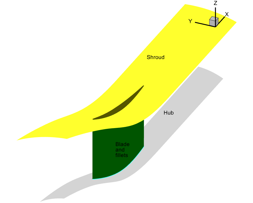
Fig. 6.8.2 TU Berlin Stator slice showing the blade, hub and shroud#
As you can see above, we have the blade, hub and shroud boundaries which are going to be noSlipWall.
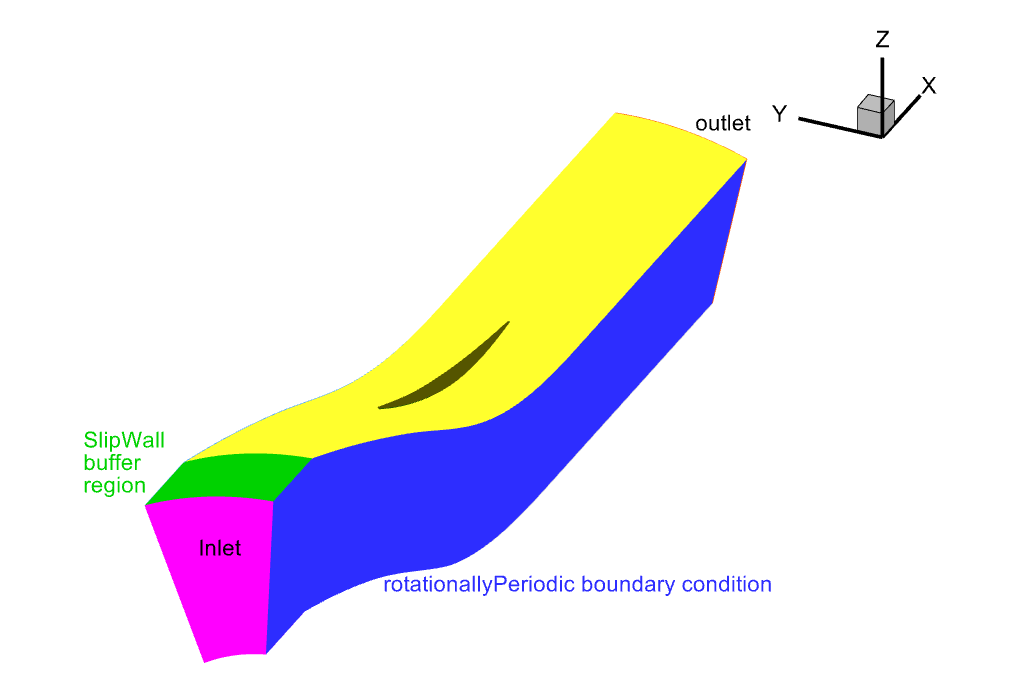
Fig. 6.8.3 Isometric view of the slice we will use as a flow domain#
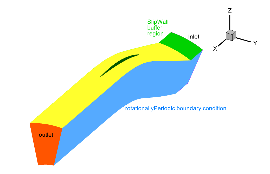
Fig. 6.8.4 Isometric view of the back of the slice we will use as a flow domain#
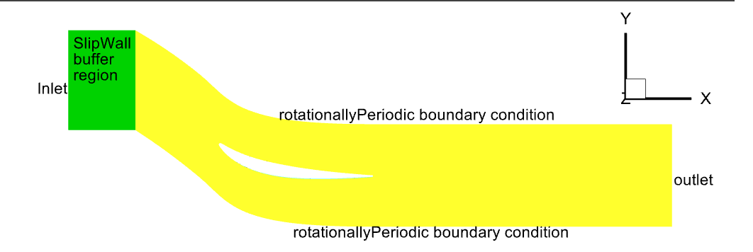
Fig. 6.8.5 top view of the slice we will use as a flow domain#
As you can see in the above top view of the flow domain, we have setup a slip wall buffer region (in green) in front of the CAD geometry (in yellow). This is a technique used to allow for better convergence. Since we have a given velocity at the inlet, when that velocity meets the noSlipWall at the hub and shroud then there will be a very large local gradient. That buffer region in green is set as a SlipWall boundary condition and it gives the code a little room to spread that large gradient and thus converge better.
Defining the boundary conditions.#
A realistic scenario would be to define a given velocity distribution across the inlet using the Freestream.velocity option but for the sake of this tutorial we will assume that the inflow is constant across the whole inlet. To that end we will simply assign the following Boundary conditions to the various regions:
operating_condition = fl.operating_condition_from_mach_reynolds(
    mach=0.13989,
    reynolds=3200,
    project_length_unit=1 * fl.u.m,
    temperature=298.25 * fl.u.K,
)
fl.SimulationParams(
    models =
    [
        fl.Wall(
            surfaces=[
                volume_mesh["fluid/vane_ss"],
                volume_mesh["fluid/vane_ps"],
                volume_mesh["fluid/bladeFillet_ss"],
                volume_mesh["fluid/bladeFillet_ps"],
                volume_mesh["fluid/shroud"],
                volume_mesh["fluid/hub"],
            ]
        ),
        fl.Freestream(
            surfaces=[
                volume_mesh["fluid/inlet"],
            ]
        ),
        fl.Outflow(
            surfaces=[
                volume_mesh["fluid/outlet"],
            ],
            spec=fl.Pressure(1.0032 * operating_condition.thermal_state.pressure),
        ),
        fl.SlipWall(
            surfaces=[
                volume_mesh["fluid/bottomFront"],
                volume_mesh["fluid/topFront"],
            ]
        ),
        fl.Periodic(
            surface_pairs=[(volume_mesh["fluid/periodic-1"], volume_mesh["fluid/periodic-2"])],
            spec=fl.Rotational(axis_of_rotation=(1, 0, 0)),
        ),
    ]
)
As you can see we have simply assigned a Freestream boundary condition at the inlet. The noSlipWall boundary condition is defined using Wall. Notice how fluid/bottomFront and fluid/topFront are set as SlipWall boundaries and how we have a small staticPressureRatio across the outlet.
Notice also how the two RotationallyPeriodic boundaries are across from each other in the above images and that we have set them as a RotationallyPeriodic pair in Periodic.surface_pairs.
The Rotational.axis_of_rotation is optional. If you know the value then it is a good idea to include it. If it is not included then the software tries to calculate the value based on the geometry of the mesh. Including it guarantees that the correct values will be used.
Once we have set the boundary conditions setting up the rest of the simulation parameters is trivial.
Case running#
After launching the case using the provided mesh and Python Script, in a few minutes, you will see the run converge and the forces quickly stabilize
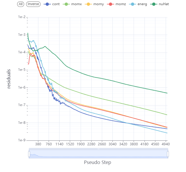
Fig. 6.8.6 Convergence plot showing more then 3 orders of magnitude decrease in the residuals.#
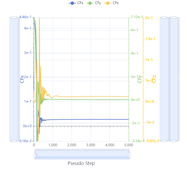
Fig. 6.8.7 Force history plot showing good convergence.#
Congratulations, you can now scale those forces and moments by 15 to get the forces and moments on all 15 blades of the TU Berlin stator.
Translational periodic boundary conditions#
Another periodic boundary condition that functions like the rotationallyPeriodic boundary condition is the translationallyPeriodic boundary condition, which can be defined using Periodic and Translational. This is useful when the periodicity is not rotational but translational. An example would be a 2D airfoil. By using a translationallyPeriodic boundary condition you could mesh a small subsection of the span and simulate an infinite span 2D section.
This is particularly useful when you want to model 3D flow structures emanating from a 2D geometry. You can see this breakdown from 2D vortices into 3D vortices in our validation study on Scale-Resolving Simulations Past a Circular Cylinder; specifically this image