Time Stepping

timeStepSize

timeStepSize prescribes the size of each physical time step.

• For steady case, the steady solver can be activated using Steady class without setting timeStepSize.

• For unsteady cases, there are two typical ways for determining the step_size:

  • Based on an expected vortex shedding frequency

  • Based on the desired angle of rotation per step

If a single volume zone with a non-zero omega is present in the simulation, setting SimulationParams.time_stepping with Steady activates a Single Reference Frame simulation. For multiple volume zones with different omega values, the Multiple Reference Frame will be used.

Vortex Shedding Frequency

The vortex shedding frequency can be estimated by:

(8.3.1)\[f = \frac{St \cdot U_\infty}{D }\]

where \(U_\infty\) is the freestream speed, \(D\) is the characteristic length, for example the mean aerodynamic chord, and \(St\) is the Strouhal Number. An approximation of \(St = 0.2\) is typically appropriate for most CFD applications.

Typically, the physical time step size \(\Delta t\) is set as:

(8.3.2)\[\Delta t = \frac{1}{100} \cdot \frac{1}{f}\]

Angle of Rotation per Step

If there is a transient BET Line or a sliding interface modeled, then the timeStepSize can be calculated from the desired angle of rotation in each physical step.

Table 8.3.1 Recommended angle of rotation per step for different scenarios.

Scenario	Angle per timeStepSize
Transient BETDisks (i.e., BET Line)	6 deg/step
Rotor in sliding interface, phase-I: Initializing the flow-field with 1st-order solver	6 deg/step
Rotor in sliding interface, phase-II: Initializing the flow-field with 2nd-order solver	6 deg/step
Rotor in sliding interface, phase-III: Collecting the data with 2nd-order solver	3 deg/step
Strong blade-vortex interaction (hover/descent)	1-2 deg/step
Generating high-quality time-resolved animation	0.5-1 deg/step

For more information about 1st versus 2nd order solution, see orderOfAccuracy. Once the angle per step is determined, then the timeStepSize can be calculated:

(8.3.3)\[\text{timeStepSize} = \theta \cdot \frac{\pi}{180} \cdot \frac{1}{\text{omegaRadians}}\]

where \(\theta\) is the angle of rotation in degrees. Note that the omegaRadians here is the nondimensional rotation speed, which can be easily converted from RPM.

maxPseudoSteps

• For steady cases, Steady.max_steps is typically 5K~10K. If the nonlinear residuals and/or the forces and moments are still changing, the user can always fork the completed case and let it run more pseudo steps.

• For unsteady time-accurate cases, max_pseudo_steps is typically slightly larger than ramp_steps so the final CFL can be achieved. As shown in the examples below, when ramp_steps = 10 then max_pseudo_steps should be set to 12. If ramp_steps = 33 then max_pseudo_steps should be set to 35.

Example time_stepping for the 1st-order unsteady cases

time_stepping = fl.Unsteady(
   max_pseudo_steps=12, CFL=fl.RampCFL(initial=1, final=1000, ramp_steps=10)
)

Example time_stepping for the 2nd-order unsteady cases

time_stepping = fl.Unsteady(
   max_pseudo_steps=35, CFL=fl.RampCFL(initial=1, final=1e7, ramp_steps=33)
)

For more information about 1st versus 2nd order solution, see orderOfAccuracy. The CFL number will be discussed in the following subsection.

CFL

The CFL number determines the pseudo step size in each physical step. Two different approaches exist in Flow360 to drive the CFL number (which are activated by setting the Steady.CFL or Unsteady.CFL):

• RampCFL, where the CFL ramping is defined by the user.

• AdaptiveCFL, where the ramping is automatically adapted based on the linear residual values.

RampCFL

The CFL ramping is defined by the user using this approach by setting values for initial , final and ramp_steps. The table below shows recommended values for CFL number ramping for steady and unsteady cases.

Table 8.3.2 Recommended CFL ramp up for steady and unsteady cases.

Example	Type	initial	final	ramp_steps
Simple wing or fuselage, mostly attached linear flow	Steady	5	200	100
Full aircraft with nonlinear flow, some separation, simple actuator/BET disks	Steady	1	100~150	1K~2K
Full aircraft near onset of stall, large-scale separation, challenging actuator/BET disks	Steady	0.1~1	10~50	3K~5K
Forked/child case	Steady	parent final CFL	parent final CFL	1
Rotor in sliding interface, 1st-order solver	Unsteady	1	1000	~10
Rotor in sliding interface, 2nd-order solver	Unsteady	1	1e+5~1e+7	30~50

1. For steady cases, initial CFL < 1, final CFL < 100, ramp_steps > 3K are considered as conservative. Such conservative values are only recommended for challenging cases.

2. For unsteady cases, it is typically recommended to let the nonlinear residuals drop 2~3 orders of magnitude in each physical step. That is why higher final CFL and more aggressive CFL ramping values are suggested.

3. For unsteady cases running 2nd-order solver, final CFL < 1e+5, ramp_steps > 50 are considered as conservative. Decreasing ramp_steps and max_pseudo_steps within each physical step will decrease the overall cost and runtime. For more information about 1st versus 2nd order solutions, see orderOfAccuracy.

AdaptiveCFL

This approach adaptively adjusts the CFL number with criteria based on the linear residual values. The AdaptiveCFL ramping approach offers several advantages when compared to RampCFL:

• The user does not need prior knowledge on the complexity of the simulation in terms of how conservatively or aggressively the CFL can be driven.

• The AdaptiveCFL will lead to faster convergence, when the user enters too conservative CFL settings in RampCFL

• The AdaptiveCFL can prevent divergence when the user enters too aggressive CFL settings in RampCFL (when the divergence is related to the time stepping settings, rather than mesh related).

• The AdaptiveCFL will lead to deeper residual convergence when the user enters too aggressive CFL settings in RampCFL, but the simulation does not diverge.

A few aspects must be noted when using AdaptiveCFL:

• The AdaptiveCFL compromises solution speed and solution robustness over a wide range of cases in terms of complexity. Therefore, the AdaptiveCFL will not necessarily lead to a faster solution than RampCFL, when the RampCFL settings are optimised.

• If the linear residuals are low (below 0.1) when divergence occurs during RampCFL, switching to AdaptiveCFL will not necessarily remedy the issue, as the CFL is adapted based on the linear residual values

As the AdaptiveCFL numerical parameters have been optimised over a range of cases in terms of complexity (from 2D aerofoil to complex 3D flows with separation and shocks), a number of optional inputs have been made available to the user to alter the AdaptiveCFL settings. These include max_relative_change, convergence_limiting_factor, min and max.

max_relative_change

The max_relative_change parameter controls the maximum relative change of the CFL number at each pseudo-step, with the default value set to 1.0. Increasing this parameter will therefore let the CFL change more rapidly, speeding up convergence but potentially leading to divergence for more complex cases. Conversely, reducing the value of this parameter constrains the relative change of the CFL number. An example of how the max_relative_change parameter affects the convergence is shown for the ONERA quick-start example, with the CFL number, non-linear and linear residuals (continuity) convergence shown in Fig. 8.3.1-Fig. 8.3.4. The max_relative_change value will affect the convergence speed without affecting the thresholds put on the linear residual in the adaptive CFL algorithm at the initial stages of the run. The same final CFL values will be reached for different max_relative_change entries at the end of the simulation (if the simulations are ran long enough). If the convergence is slower than expected RampCFL settings, it is recommended to increase the max_relative_change value.

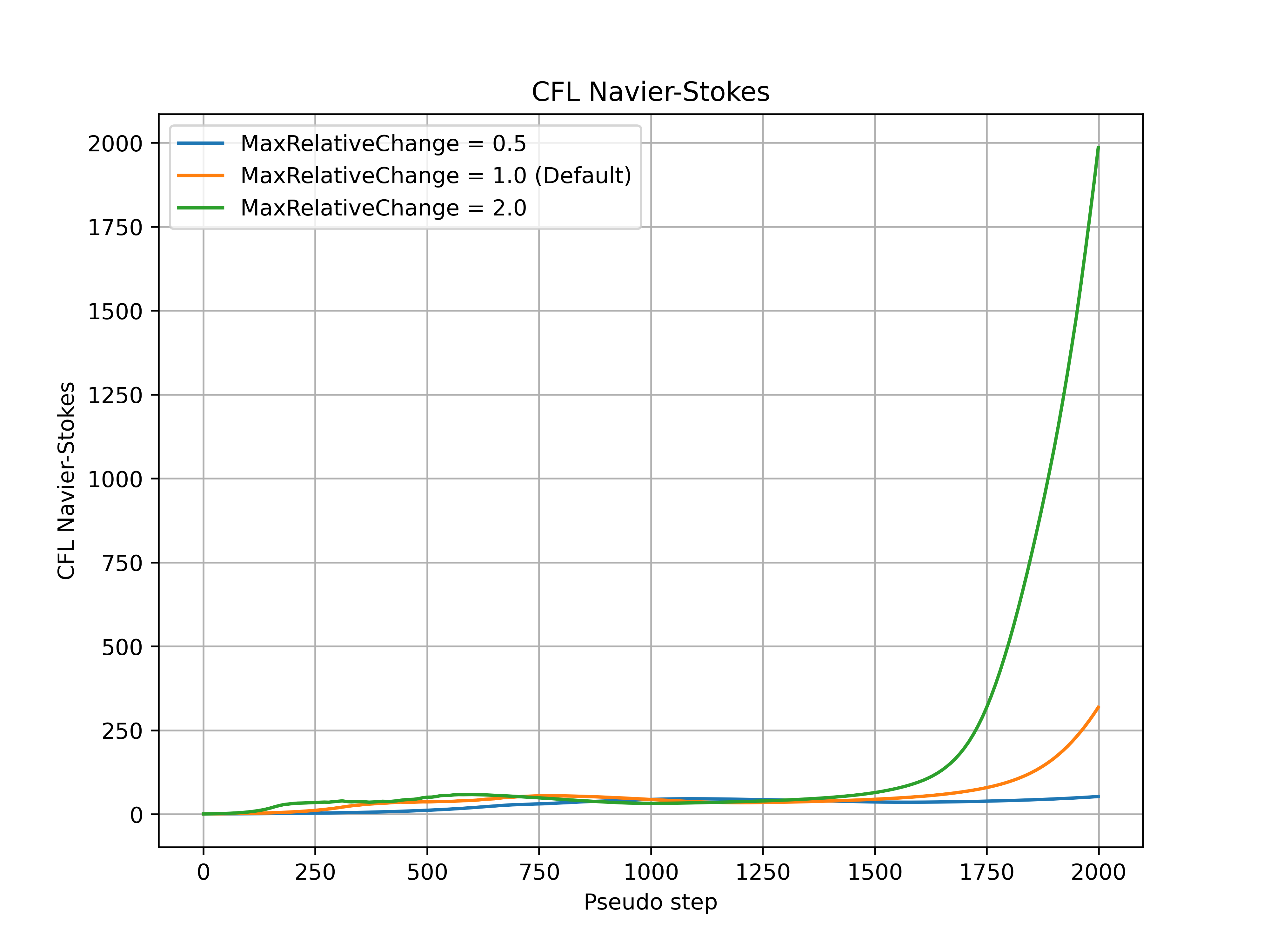
Fig. 8.3.1 Navier-Stokes CFL number during the simulation for a range of max_relative_change values.

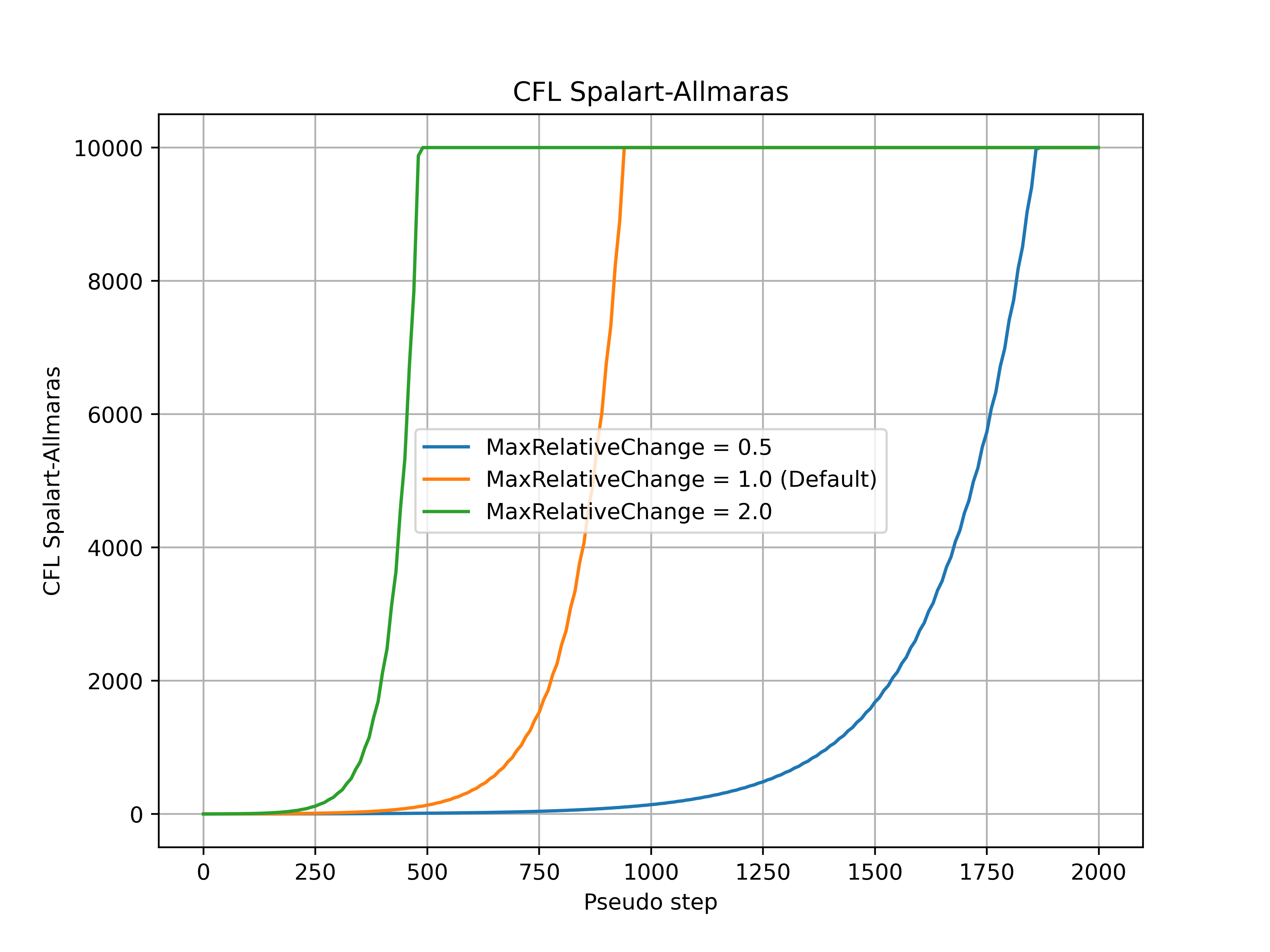
Fig. 8.3.2 Spalart-Allmaras CFL number during the simulation for a range of max_relative_change values.

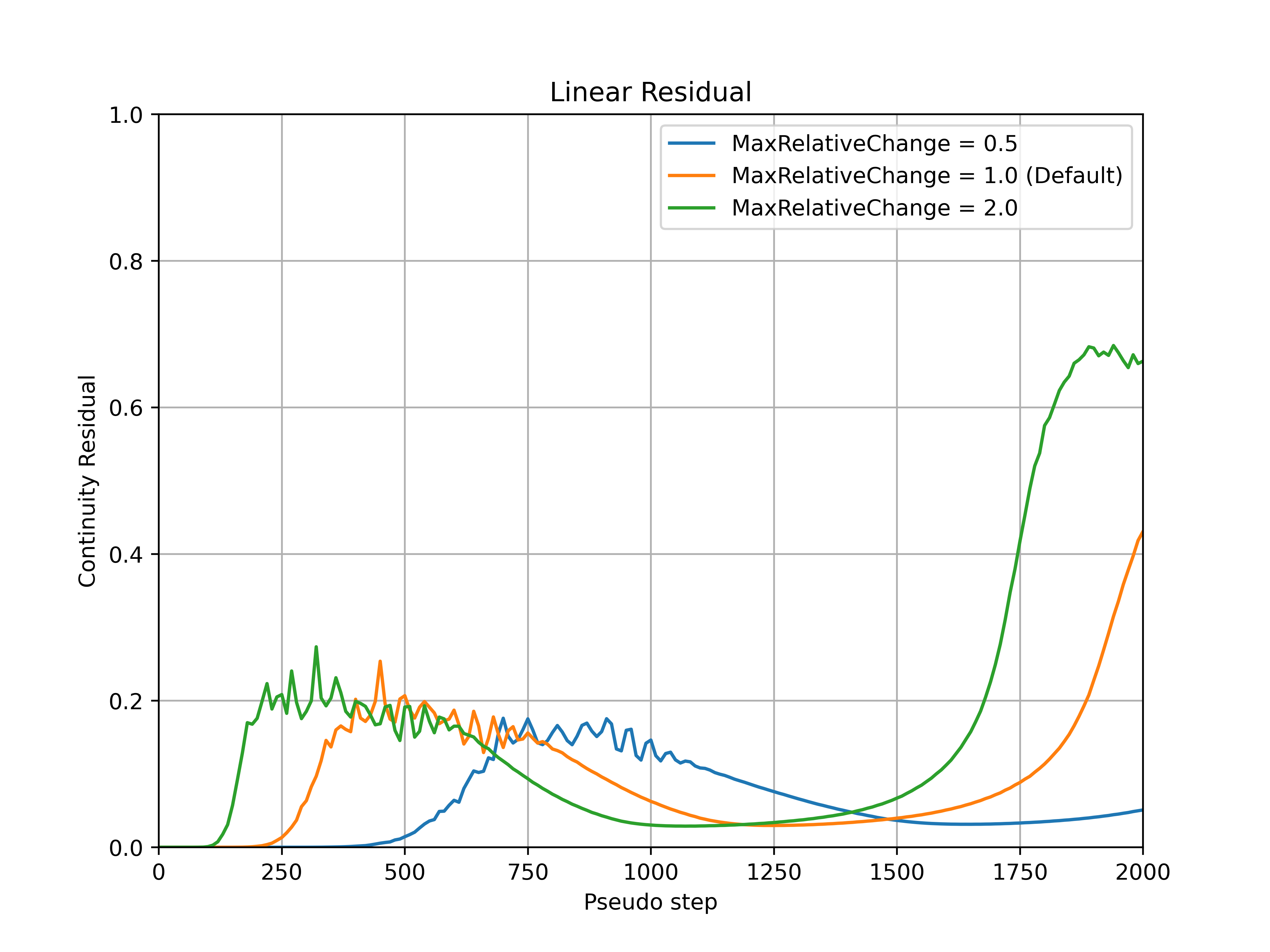
Fig. 8.3.3 Continuity linear residual convergence during the simulation for a range of max_relative_change values.

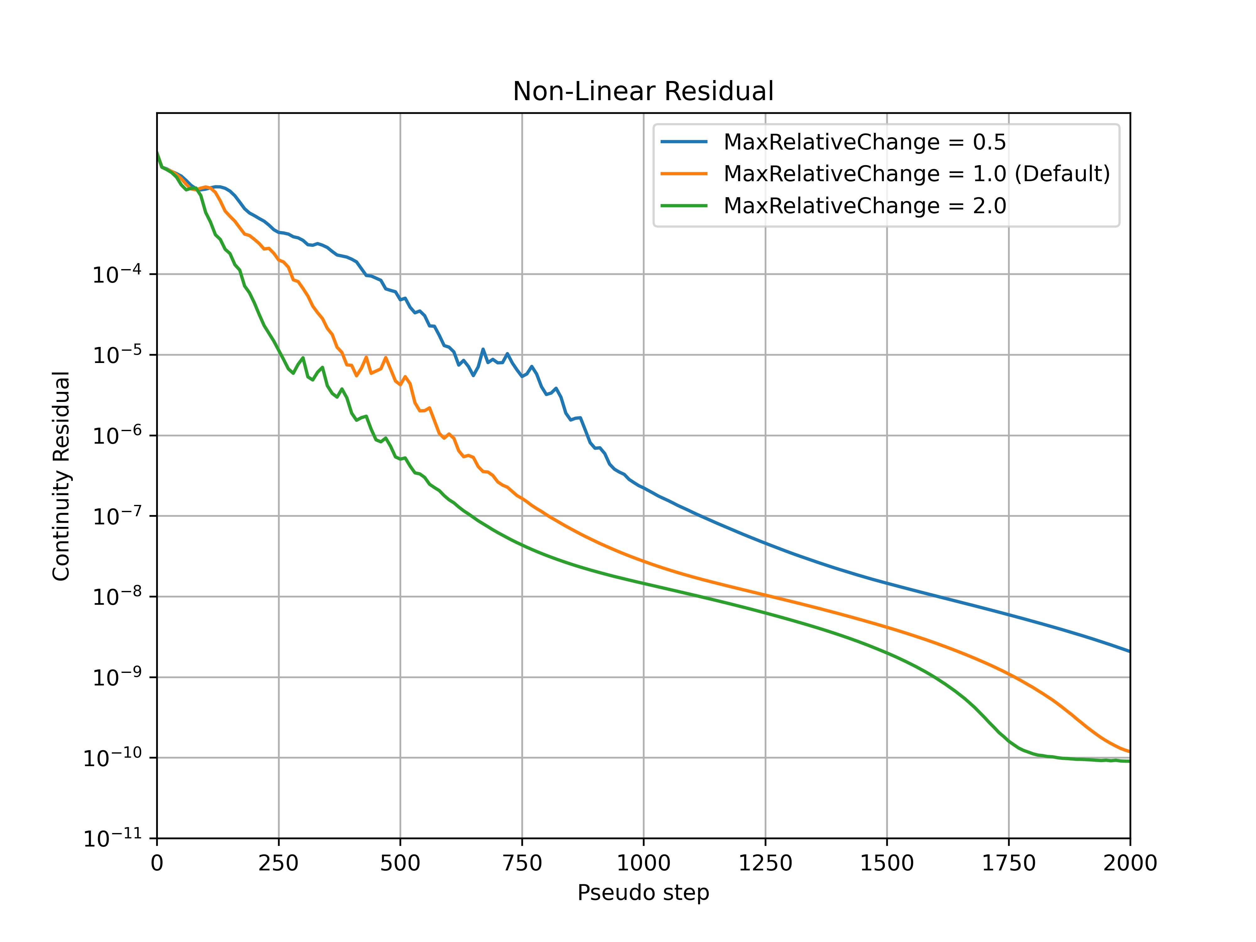
Fig. 8.3.4 Continuity non-linear residual convergence during the simulation for a range of max_relative_change values.

convergence_limiting_factor

The convergence_limiting_factor modifies how conservative or aggressive the limitations on the values of CFL are. Smaller convergence_limiting_factor values lead to a more conservative CFL value, whereas larger convergence_limiting_factor values lead to a more aggressive CFL value. The default value is set to 0.25 which is a good compromise between solution speed and robustness across a wide range of cases. An example of how the convergence_limiting_factor parameter affects the convergence is shown for the ONERA quick-start example, with the CFL number, non-linear and linear residuals (continuity) convergence shown in Fig. 8.3.5-Fig. 8.3.8. The convergence_limiting_factor does not affect the initial CFL values (under 250 pseudo-steps in this case), but has an impact on the thresholds of the linear residuals during the adaptive CFL algorithm and CFL numbers reached in the later stages of the simulation. Higher values of convergence_limiting_factor lead to faster convergence of the nonlinear residual but also permit higher values of the linear residual during the simulation. In the case of simulation divergence, it is recommended to reduce the value of convergence_limiting_factor (after checking the mesh quality at the divergence location, see Fixing Divergence Issues.

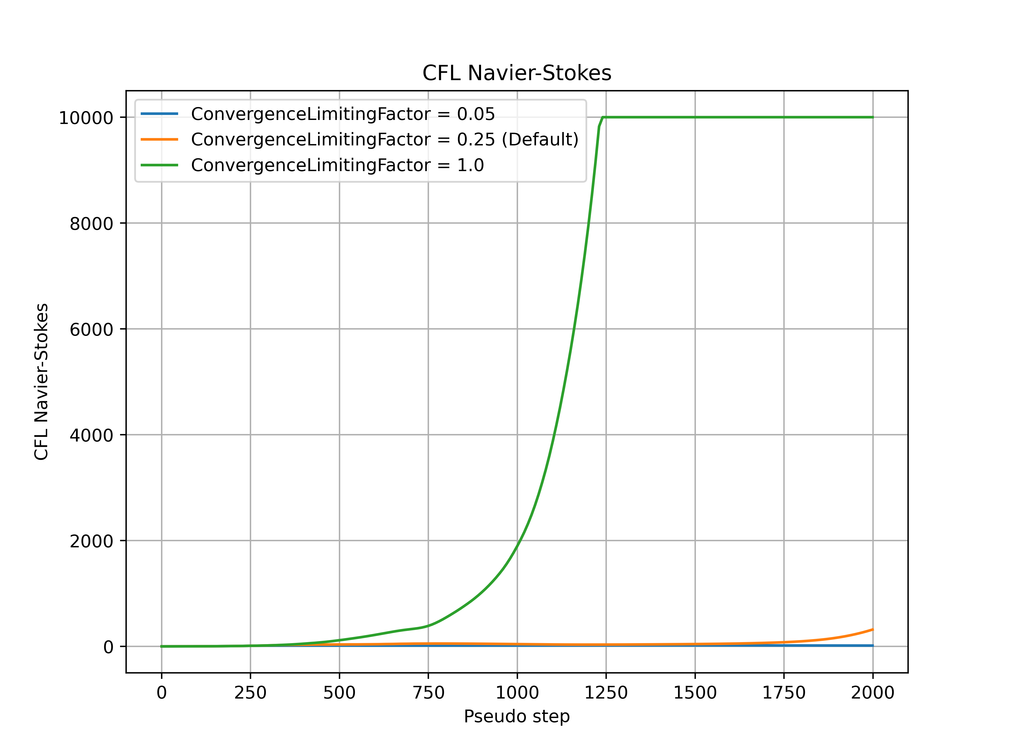
Fig. 8.3.5 Navier-Stokes CFL number during the simulation for a range of convergence_limiting_factor values.

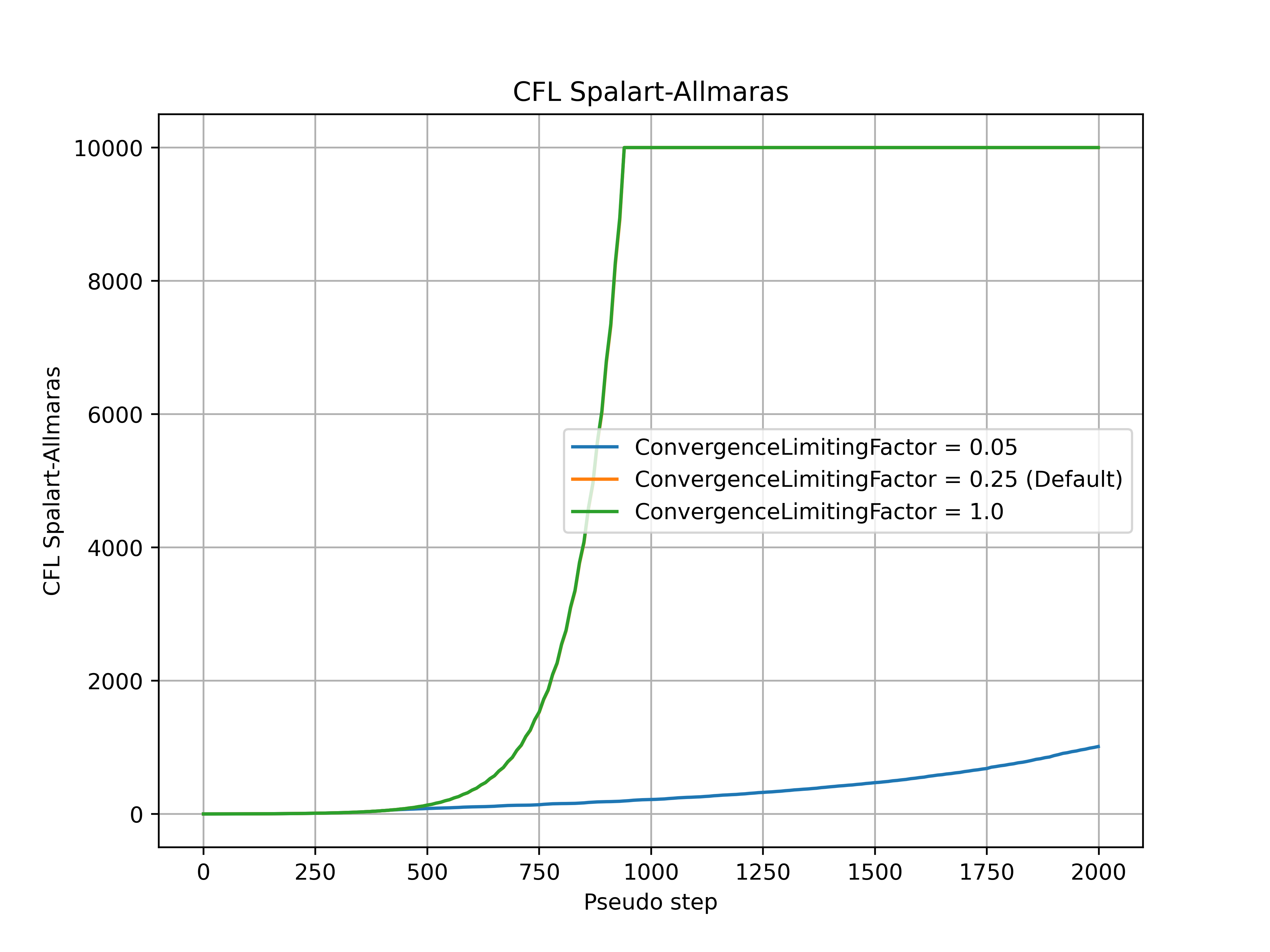
Fig. 8.3.6 Spalart-Allmaras CFL number during the simulation for a range of convergence_limiting_factor values.

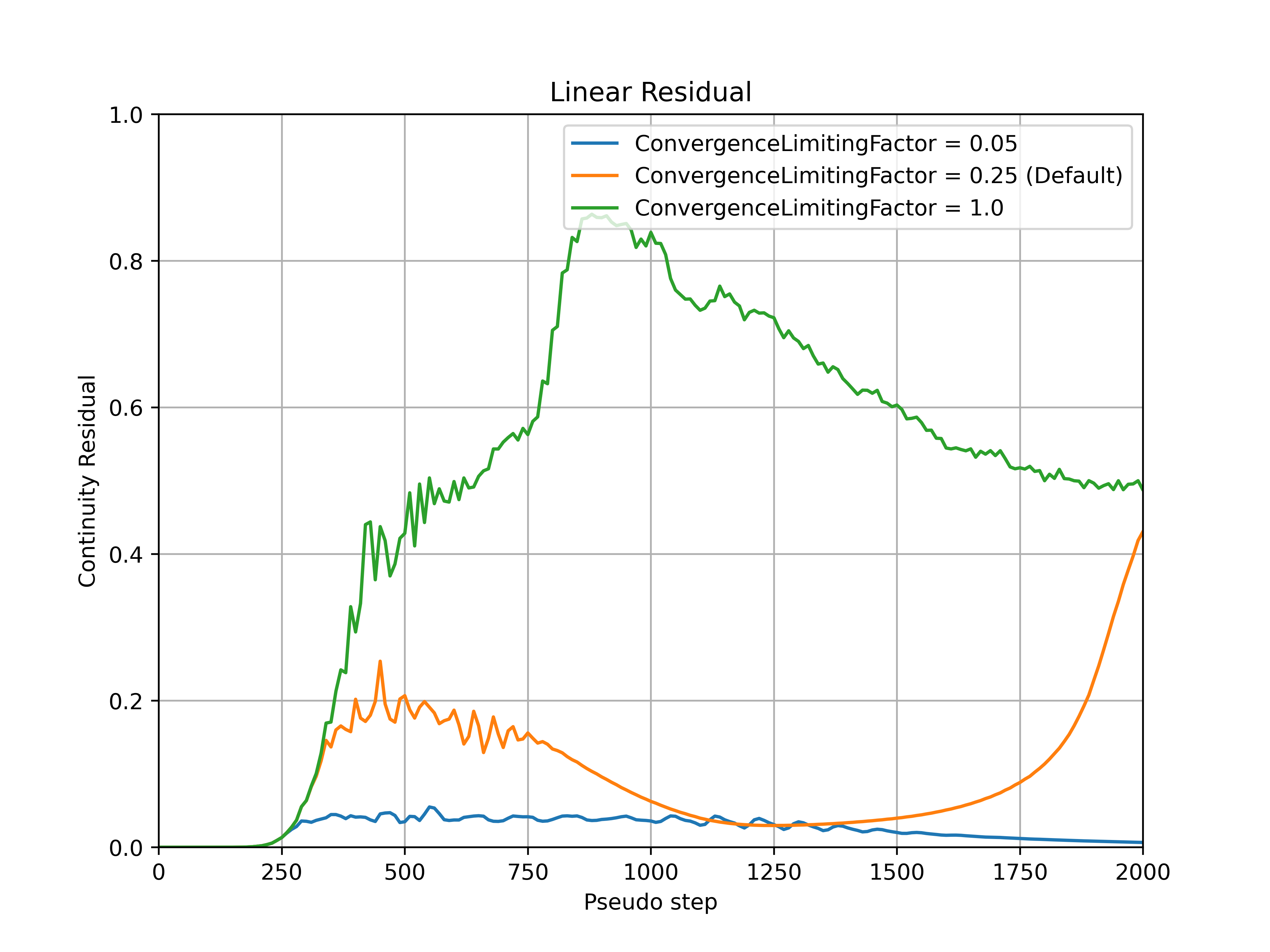
Fig. 8.3.7 Continuity linear residual convergence during the simulation for a range of convergence_limiting_factor values.

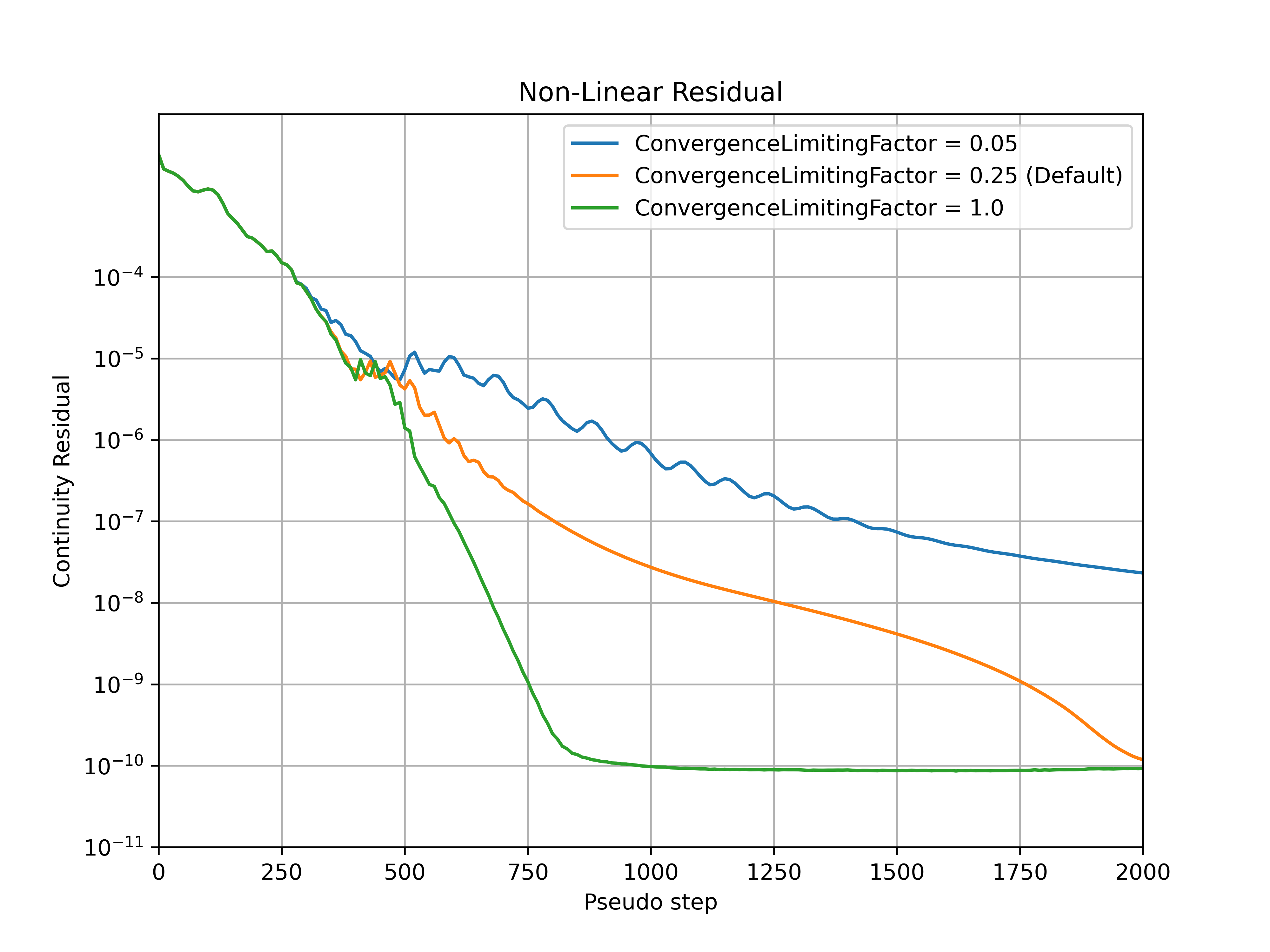
Fig. 8.3.8 Continuity non-linear residual convergence during the simulation for a range of convergence_limiting_factor values.

min

The min parameter affects the minimum values of the CFL number for the solved equations during the simulation.

max

The max parameter affects the maximum values of the CFL number for the solved equations during the simulation. An example use case for when this parameter would need to be modified is when the Spalart-Allmaras solver diverges with a non-physical turbulent eddy viscosity. As the Spalart-Allmaras is a one-equation model compared to the five equations that are solved for the Navier-Stokes solver, the linear residuals for the Spalart-Allmaras solution will usually be much lower, and therefore the CFL will be driven to much higher values, which may prompt reducing the max allowable CFL during the adaptive CFL algorithm.

Comparison between RampCFL and AdaptiveCFL

A comparison of the RampCFL and AdaptiveCFL approaches was performed for the ONERA quick-start example example for a range of settings, with the CFL number, non-linear and linear residuals (continuity) convergence shown in Fig. 8.3.9-Fig. 8.3.12.

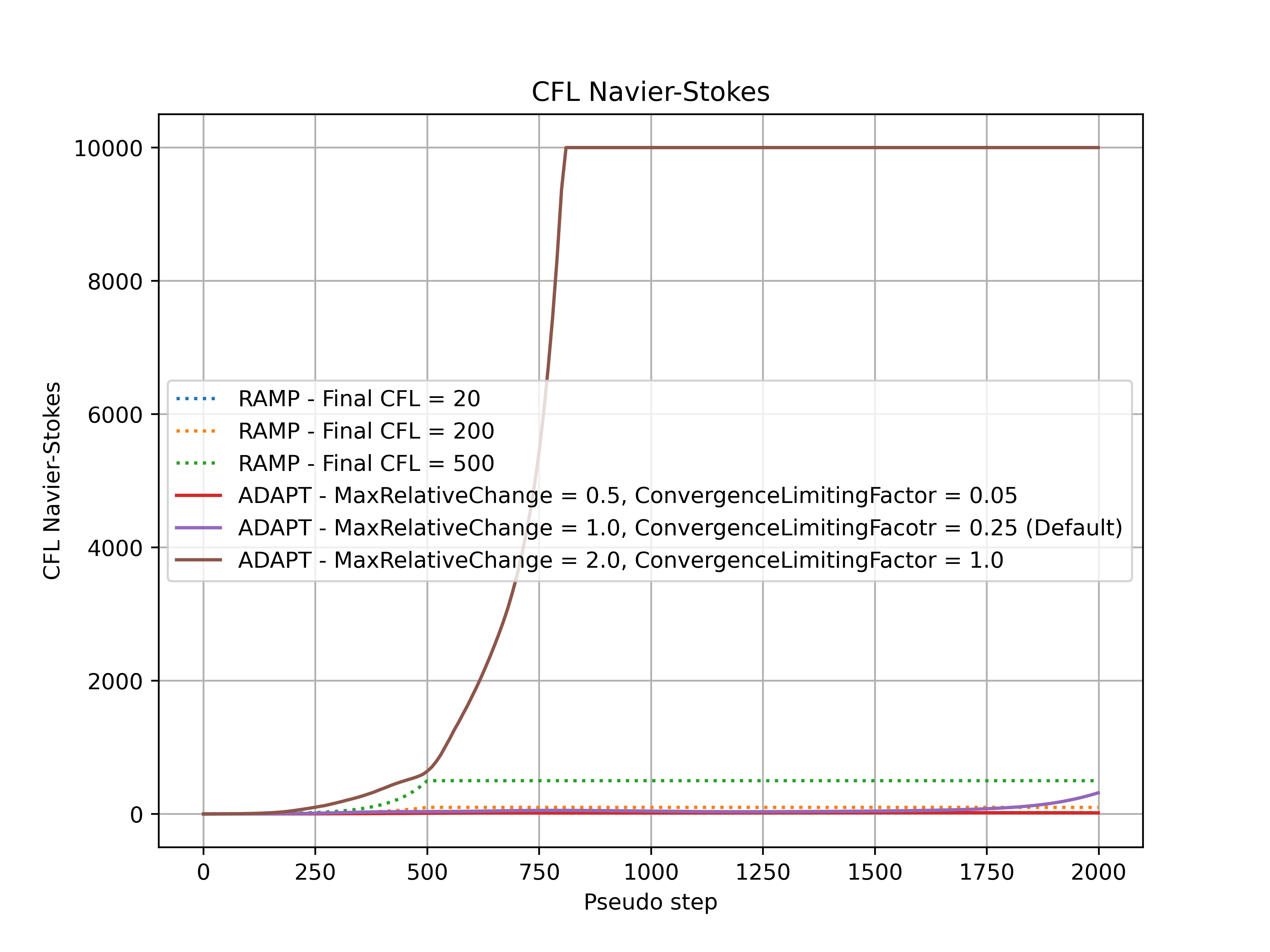
Fig. 8.3.9 Comparison of the Navier-Stokes CFL number during the simulation for adaptive and ramped CFL.

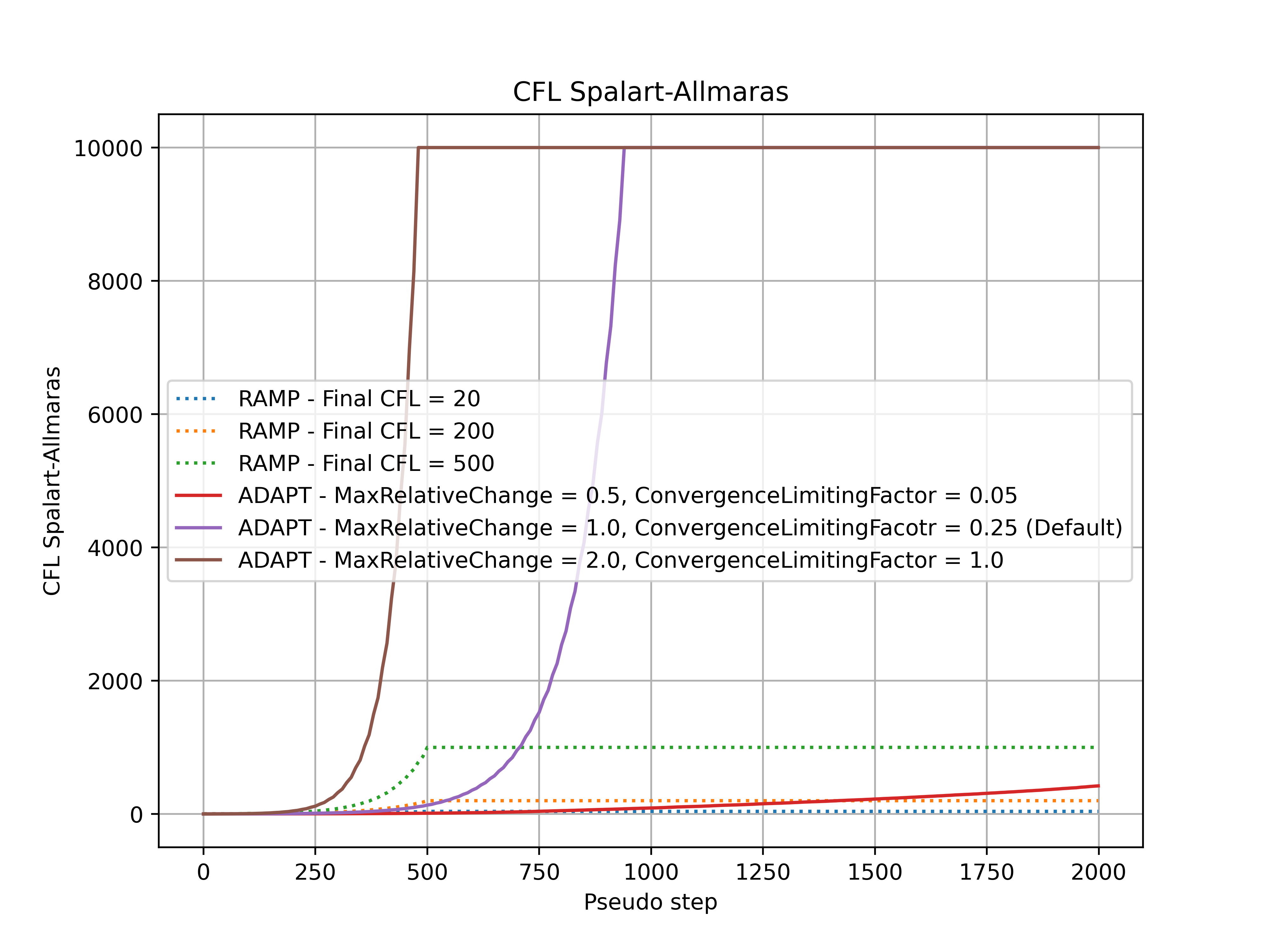
Fig. 8.3.10 Comparison of the Spalart-Allmaras CFL number during the simulation for adaptive and ramped CFL.

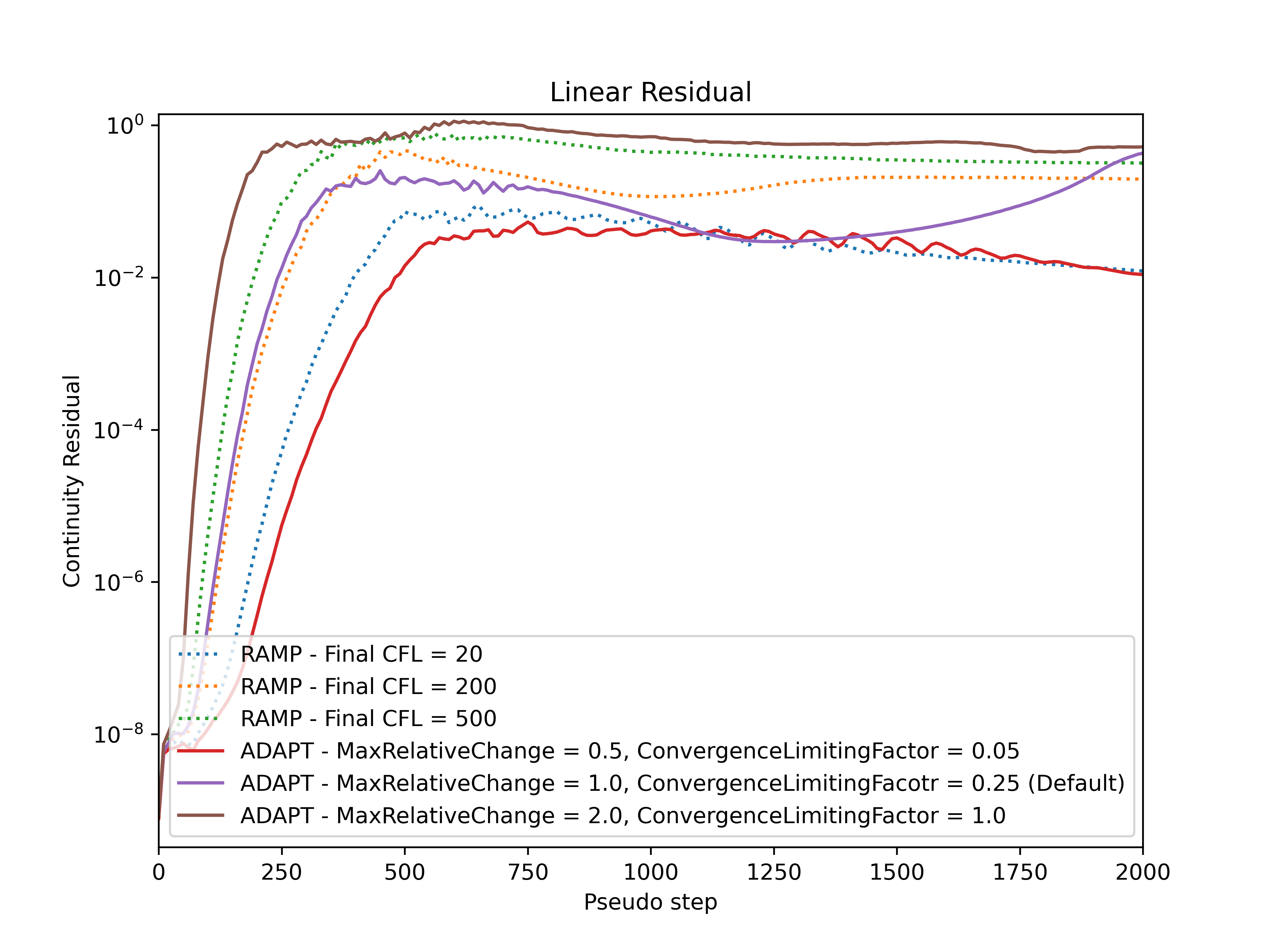
Fig. 8.3.11 Comparison of the continuity linear residual convergence during the simulation for adaptive and ramped CFL.

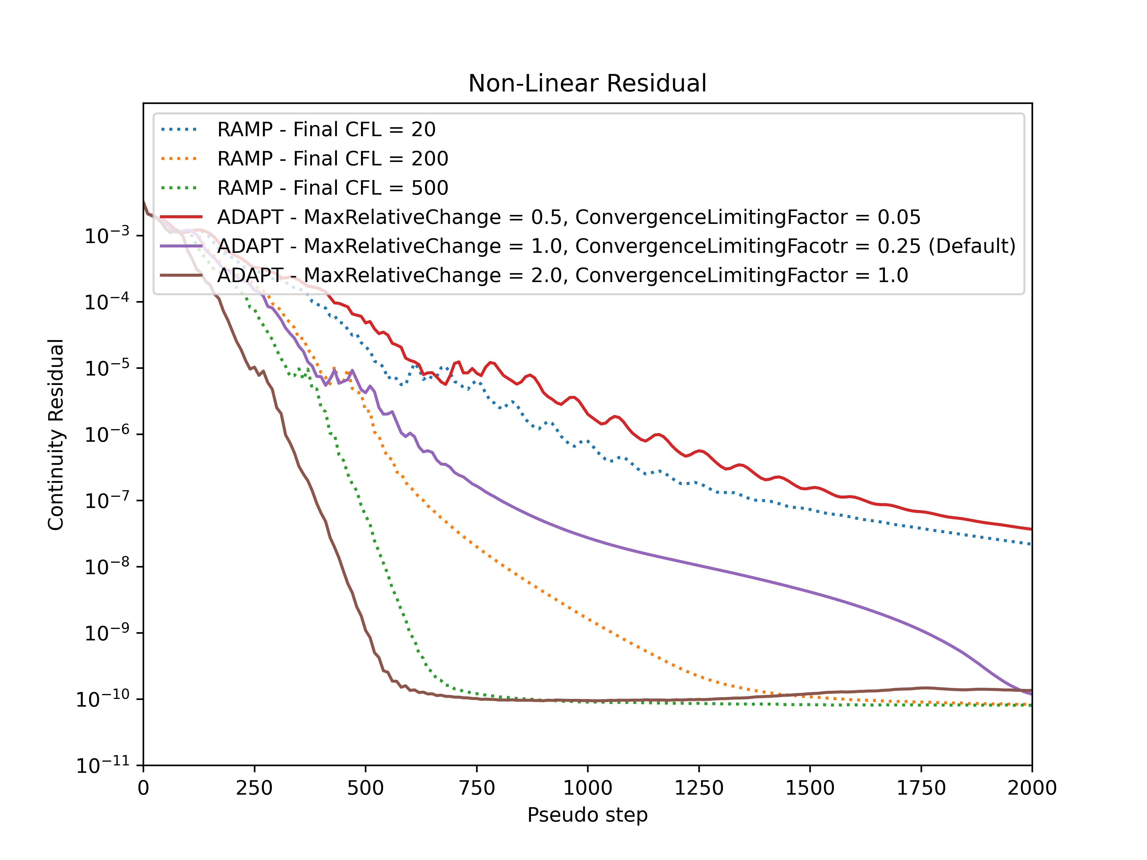
Fig. 8.3.12 Comparison of the continuity nonlinear residual convergence during the simulation for adaptive and ramped CFL.

Firstly, it must be noticed that divergence is not a key limiter in the CFL values used in this example. For an example where adaptive CFL is used to prevent divergence, see Fixing Divergence Issues. It can be seen that the CFL values at the end of the simulation and convergence speed are driven by the RampCFL.final and AdaptiveCFL.convergence_limiting_factor for both algorithms. The adaptive CFL algorithm allows for much higher Spalart-Allmaras CFL values. In general similar behaviour is seen between the RampCFL and AdaptiveCFL, with less conservative settings leading to faster convergence and higher linear residual values. The key benefit of the AdaptiveCFL algorithm is that the CFL will automatically be reduced when the linear residuals are above a given threshold, in many cases preventing divergence.