7.4. User Defined Expressions

Variables

Variable (also known as custom variable or UserVariable) is a user-defined concept that utilizes expressions to define their value. The expression defines the variable’s value and can involve mathematical operations using constants (such as numbers or vectors), units (like u.m), and other variables.

Variables can be used as inputs to a simulation or for post-processing. For more details, see the Expressions section.

Table 7.4.1 Example Variables

Name	Expression
velocity_ref	100.0 * u.m / u.s
rho	1.225 * u.kg / u.m**3
q_inf	0.5 * rho * velocity_ref**2

Post-processing output variables are used to define outputs such as Surface output, Volume output, etc. These variables are defined by selecting the unit system in which the solution namespace variables will be output, and providing an expression that will define the post-processing variable.

A simple example of setting up post-processing output variables is shown below.

First, we define a my_velocity_magnitude variable.

math.sqrt(solution.velocity[0]**2 + solution.velocity[1]**2 + solution.velocity[2]**2)

Then, we can create my_dynamic_pressure based on the previously defined my_velocity_magnitude.

0.5 * solution.density * my_velocity_magnitude**2

If we assume that the project for which these variables are defined, was assigned the SI unit system, my_velocity_magnitude and my_dynamic_pressure will have values scaled to meters per second and Pascals, respectively.

More details about units and dimensionality are provided in the Expressions section. Solution variables and math operations are listed in their respective sections Solution Variables and Math Operations.

Variables can also be created and utilized with the help of Python API. Below is a short example of how to create and use variables.

import flow360 as fl
my_vel = fl.UserVariable(name="velocity_input", value=50 * fl.u.m / fl.u.s)
fl.AerospaceCondition(velocity_magnitude=my_vel)

my_temp = fl.UserVariable(name="temperature_rankine", value=fl.solution.temperature).in_units(new_unit="R")
fl.ProbeOutput(
    name="probe_output",
    output_fields=[my_temp],
    probe_points=[fl.Point(name="point_1", location=(1, 1, 1) * fl.u.m)],
)

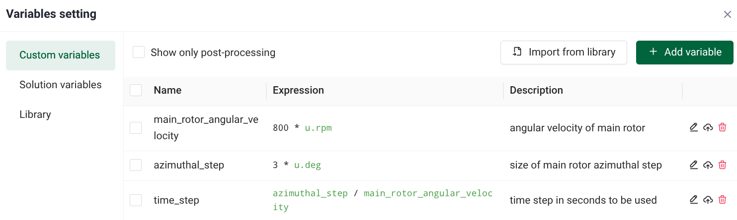
As a more complex example, we will show how to set up the time step to match a desired rotor azimuthal rotation in degrees per step. We start by defining angular velocity of the rotor main_rotor_angular_velocity,

800 * u.rpm

and the azimuthal step azimuthal_step.

3 * u.deg

Afterwards we can use these variables to define the time step as time_step.

azimuthal_step / main_rotor_angular_velocity

This results in 3 variables in total, which can be checked in the Custom variables tab in the UI.

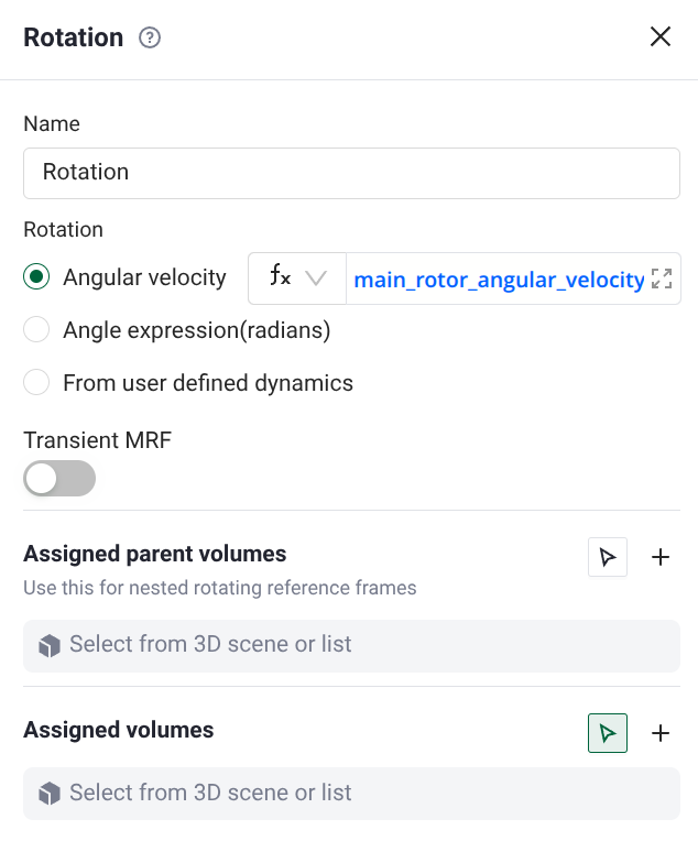
Once we have all the variables defined, we can use them in the simulation setup. Rotor speed is set here.

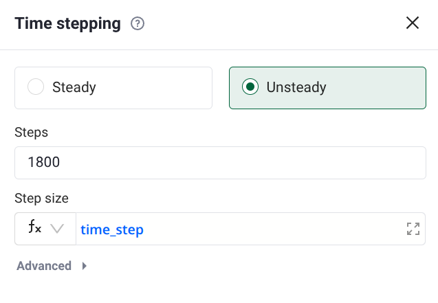
The total number of steps is computed manually using the following formula.

total_number_of_steps = 15 * 360 * u.deg / azimuthal_step = 1800

For 15 revolutions and a 3 degree step size the total number of steps is 1800. Finally, the time settings can be set as shown below.

Expressions

Expressions in Flow360 are symbolic dimensioned mathematical representations that allow you to create complex calculations using variables, constants, mathematical functions, and operators. They provide a way of defining post-processing variables, and input parameters for your simulations.

What is important to keep in mind when using expressions is the dimensionality. For example, velocity magnitude field expects dimensions of (length) / (time) and step size field (in unsteady) expects dimension of (time).

# Correct velocity magnitude dimensions (length per time)

50 * u.m / u.s

# Wrong velocity magnitude dimensions (length per time squared)
50 * u.m / u.s**2

# Wrong velocity magnitude dimensions (dimensionless)
50

This should also be considered during the definition of post-processing output variables.

Main difference here is that for input expressions (or input variables that use expressions) Flow360 will check whether they have correct dimensions, but for post-processing variables that is not the case. Due to that, double checking the correct dimensionality is recommended when setting up post-processing variables.

Units

Units are essential for ensuring dimensional consistency and proper physical calculations in your expressions. Flow360 uses the unyt package to provide unit support in user-defined expressions, more information can be found in the unyt documentation. Units are accessed through the u namespace and can be combined using standard mathematical operations:

# Basic unit syntax
u.m          # meters
u.m / u.s    # meters per second (velocity)
u.kg / u.m**3  # kilograms per cubic meter (density)

Note

• Make sure that your expressions used for inputs, have not only correct dimensions, but also correct units, because they will affect the simulation itself.

• Relative temperature scales (u.degF, u.degC) are not allowed, use absolute temperature scales (u.R or u.K) instead.

Solution Variables

The outputs from the solver can be used to create variables. Currently available solution variables can be found under the solution namespace and consist of:

Name	Defined on	Description	Availability
solution.coordinate	Volume mesh	Node coordinates in the domain	Always available
solution.Cp	Volume mesh	Pressure coefficient	Always available
solution.Cpt	Volume mesh	Total pressure coefficient	Always available
solution.grad_density	Volume mesh	Gradient of density	Always available
solution.grad_u	Volume mesh	Gradient of velocity component in x-direction	Always available
solution.grad_v	Volume mesh	Gradient of velocity component in y-direction	Always available
solution.grad_w	Volume mesh	Gradient of velocity component in z-direction	Always available
solution.grad_pressure	Volume mesh	Gradient of pressure	Always available
solution.Mach	Volume mesh	Local Mach number	Not available with liquid materials
solution.mut	Volume mesh	Eddy viscosity	Always available
solution.mut_ratio	Volume mesh	Ratio of eddy to molecular viscosity	Always available
solution.nu_hat	Volume mesh	Modified kinematic viscosity for transition modeling	Requires Spalart-Allmaras turbulence model
solution.turbulence_kinetic_energy	Volume mesh	Turbulent kinetic energy (k)	Requires k-omega SST turbulence model
solution.specific_rate_of_dissipation	Volume mesh	Specific dissipation rate (ω or ε)	Requires k-omega SST turbulence model
solution.amplification_factor	Volume mesh	Amplification factor (used in transition models)	Requires amplification factor transition model
solution.turbulence_intermittency	Volume mesh	Turbulence intermittency factor	Requires amplification factor transition model
solution.density	Volume mesh	Fluid density	Not available with liquid materials
solution.velocity	Volume mesh	Velocity vector	Always available
solution.pressure	Volume mesh	Static pressure	Always available
solution.qcriterion	Volume mesh	Q-criterion for vortex detection	Always available
solution.entropy	Volume mesh	Flow entropy	Always available
solution.temperature	Volume mesh	Static temperature	Not available with liquid materials
solution.vorticity	Volume mesh	Vorticity vector	Always available
solution.wall_distance	Volume mesh	Distance to the nearest wall (used in turbulence models)	Always available
solution.CfVec	Surface mesh	Skin friction vector	Always available
solution.Cf	Surface mesh	Skin friction coefficient	Always available
solution.heatflux	Surface mesh	Heat flux at surface	Always available
solution.node_area_vector	Surface mesh	Surface area vector per node	Always available
solution.node_unit_normal	Surface mesh	Unit normal vector at surface node	Always available
solution.node_forces_per_unit_area	Surface mesh	Surface force per unit area at each node	Always available
solution.y_plus	Surface mesh	Non-dimensional wall distance (y⁺) used in turbulence models	Always available
solution.wall_shear_stress_magnitude	Surface mesh	Magnitude of wall shear stress	Always available
solution.heat_transfer_coefficient_static_temperature	Surface mesh	Heat transfer coefficient based on static temperature	Always available
solution.heat_transfer_coefficient_total_temperature	Surface mesh	Heat transfer coefficient based on total temperature	Always available

Math Operations

The following math operations can be applied to manipulate the variables definitions:

Operation	Description	Example	Supports vector input	Works with dimensioned input
+	Addition	3 + 2 = 5	✓	✓
-	Subtraction	5 - 2 = 3	✓	✓
*	Multiplication	4 * 3 = 12	✓	✓
/	Division	10 / 2 = 5	✓	✓
math.add(a, b)	Returns a + b	math.add(3, 2) = 5	✓	✓
math.subtract(a, b)	Returns a - b	math.subtract(5, 2) = 3	✓	✓
math.sqrt(x)	Square root of x	math.sqrt(9) = 3	✗	✓
math.log(x)	Natural logarithm (ln) of x	math.log(1) = 0	✗	✗
math.exp(x)	e to the power of x	math.exp(1) ≈ 2.718	✗	✗
math.sin(x)	Sine of angle x (in radians)	math.sin(π/2) = 1	✗	✗
math.cos(x)	Cosine of angle x (in radians)	math.cos(0) = 1	✗	✗
math.tan(x)	Tangent of angle x (in radians)	math.tan(0) = 0	✗	✗
math.asin(x)	Arcsine of x, result in radians	math.asin(1) = π/2	✗	✗
math.acos(x)	Arccosine of x, result in radians	math.acos(1) = 0	✗	✗
math.atan(x)	Arctangent of x, result in radians	math.atan(1) = π/4	✗	✗
math.max(a, b)	Returns the maximum of a and b	math.max(3, 5) = 5	✗	✓
math.min(a, b)	Returns the minimum of a and b	math.min(3, 5) = 3	✗	✓
math.abs(x)	Absolute value of x	math.abs(-4) = 4	✗	✓
math.cross(a, b)	Cross product of 3D vectors a and b	math.cross([1,0,0],[0,1,0]) = [0,0,1]	✓ (vectors only)	✓
math.dot(a, b)	Dot product of vectors a and b	math.dot([1,2,3],[4,5,6]) = 32	✓ (vectors only)	✓
math.magnitude(v)	Magnitude (length) of vector v	math.magnitude([3,-4,12]) = 13	✓ (vectors only)	✓
math.pi	Constant π ≈ 3.14159	math.pi ≈ 3.14159	✗	✗ (π is dimensionless)

Some operators are restricted and cannot be used in expressions. These are:

• The ^ operator is not allowed (use ** for power)

• The & operator is not allowed

Variable Name Limitations

Variable names must follow these rules:

• Start with a letter (A-Z, a-z) or underscore (_)

• Contain only letters, digits, and underscores

• Not conflict with reserved keywords or solver variable names

• Be unique within your project

Table 7.4.2 Variable Name Examples

Valid Names	Invalid Names
Mach_number	123invalid (starts with number)
wing_area	for (is a reserved keyword)
_pressureRatio	area-size (contains “-” which is not allowed)

Common Errors

Flow360 automatically validates expressions to ensure that they are correct and have proper physical meaning. This is done by checking the syntax, semantic and feature dependencies. Some of the most common errors as well as their solutions are listed below.

Table 7.4.3 Common Errors and Solutions

Error Type	Description	Solution
Undefined Variable References	Occurs when referencing a variable that hasn’t been defined	Check variable names for typos and ensure all variables are defined earlier in your setup
Unit Mismatch	Occurs when combining quantities with incompatible units	Review expressions to ensure all terms have compatible units (e.g., only add/subtract quantities with same dimensions)
Invalid Variable Names	Occurs when using reserved names or invalid identifiers	Choose unique variable names that don’t conflict with reserved keywords or solver variable names