5.13. Underwater Flow Around the DARPA Model 4740 Submarine

Introduction

This validation study aims to assess the accuracy of Flexcompute’s Flow360 solver in predicting incompressible fluid behavior.

Computational Fluid Dynamics simulations are essential in the design of maritime systems and underwater vehicles, offering a cost-effective and scalable alternative to experimental testing. Although Flow360 is primarily designed as a compressible flow solver, its ability to accurately model incompressible flows is critical for simulating liquid environments, such as those encountered in submerged applications.

To evaluate this capability, we perform a benchmark study based on the fully appended, straight-line, captive-model experiment of the DARPA Suboff (DTRC Model 4740) at deep submergence. The DARPA Suboff is a widely accepted standard for submarine validation cases and has been extensively used in both academic and industrial CFD research. Its established experimental dataset [1] [2] makes it an ideal candidate for assessing the accuracy and robustness of Flow360.

The results from Flow360 are compared to experimental measurements conducted by the Naval Surface Warfare Center as part of a DARPA-sponsored research initiative.

To guide the reader through the validation process, this document is structured into the following sections:

1. Geometry and Setup – Overview of the model geometry and experimental configuration.

2. Meshing Strategy – Description of the meshing approach and refinement techniques.

3. Simulation Parameters – Details of solver settings and boundary conditions.

4. Results and Validation – Comparison of simulation results with experimental data.

Geometry and Setup

The DARPA DTRC Model used in this case study is Model 4740 in its AFF8 configuration [1]. The geometry features an axisymmetric hull, a sail without forward control planes, and a conventional cruciform stern with four identical control surfaces. The submarine model has a total length of 4356 mm and a beam, the largest transverse cross-sectional diameter, of 508 mm. The length between perpendiculars is 4261 mm.

As a standardized geometry, all principal dimensions, reference measurements, and parametric definitions of the model are publicly available. This standardization minimizes potential sources of error arising from geometric discrepancies between the numerical model and the experimental setup, thereby providing a reliable foundation for validation.

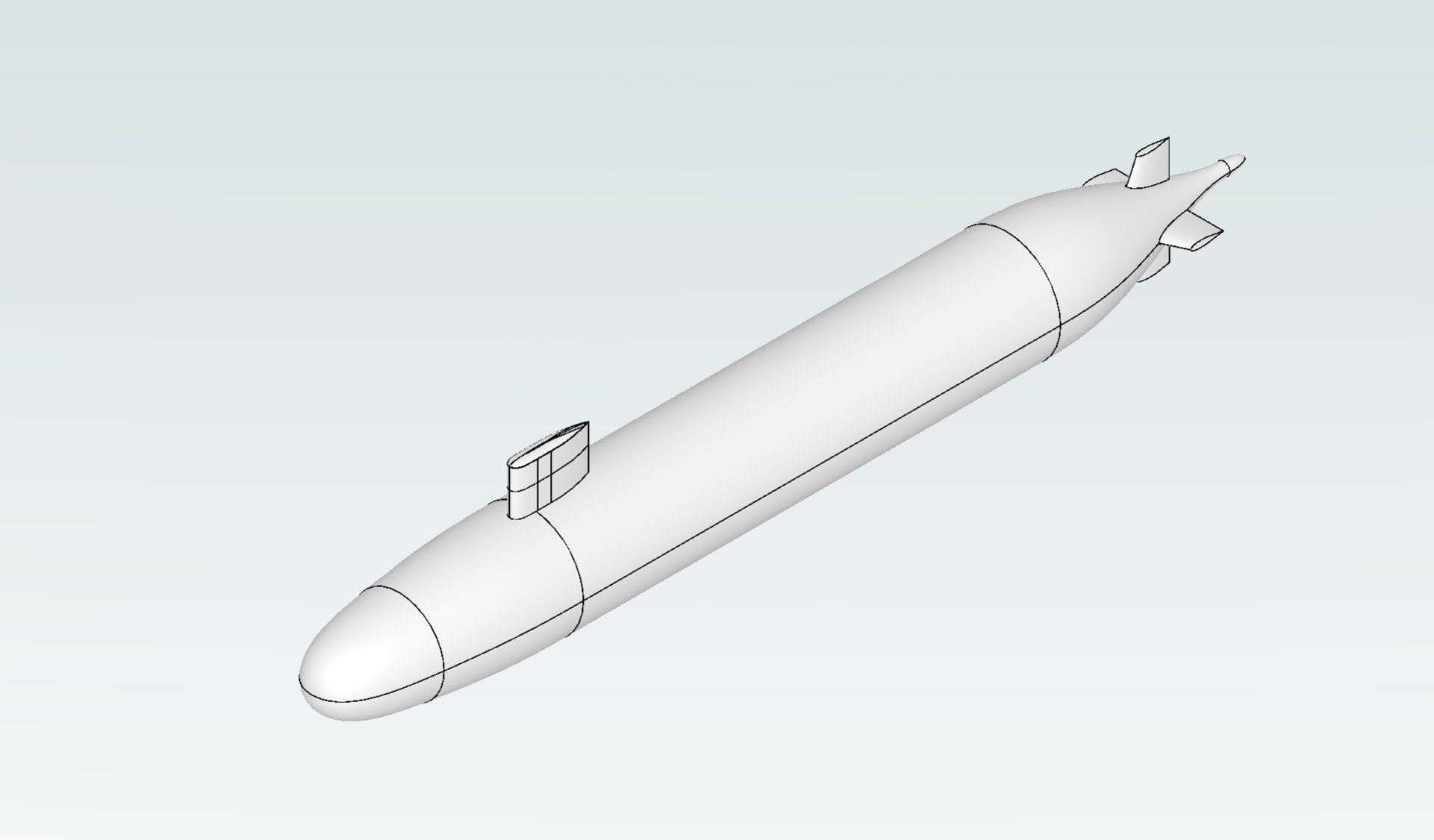
Fig. 5.13.1 DARPA 4740 Suboff geometry used for this study.

Meshing Strategy

The CAD model was meshed to ensure that all relevant flow phenomena are accurately captured, three key objectives were established during the mesh definition process:

1. A maximum surface edge length was defined to provide at least the recommended 200 points along the submarine’s waterline. Ensuring the capture of the flow phenomena along the waterline of the ship.

2. The first layer thickness was calculated using flat plate theory to target a \(y^{+}\) value close to 1 across the submarine’s surface. However, a perfectly uniform \(y^{+}\) cannot be guaranteed, as the Reynolds number, and consequently the skin friction coefficient, varies across the geometry. To ensure the mesh is sufficiently fine across all simulation cases, which involve varying flow speeds, the first layer thickness was set based on the highest velocity considered. This guarantees \(y^{+} \approx 1\) even under the most demanding flow conditions.

3. Additional surface and volume refinements were applied to ensure accurate resolution of the boundary layer along the sail and stern planes.

Finally, a uniform volume refinement was introduced within a box region extending five submarine lengths along its waterline and spanning a width three times the submarine’s diameter.

Final meshing parameters used in each case can be seen in the figure:

Table 5.13.1 Meshing Parameters

Section	Parameter	Coarse	Fine	Units
Surface mesh	Surface edge growth rate	1.2	1.1	—
	Surface max edge length	11	5.5	mm
	Max Curvature resolution angle	5	5	°
Volume mesh	Boundary layer growth rate	1.2	1.15	—
	Boundary layer first layer thickness	2	2	μm
Surface Refinements	Planar face tolerance	1e-6	1e-6	—
	Uniform refinement spacing	50	25	mm
	Stern and Sails surface max edge length	2.5	2.5	mm
	Sterns and Sails TEs max edge length		0.25	mm
	Sterns and Sails LEs max edge length		0.25	mm
Volume Refinements	Sail volume refinement	5	5	mm
	Sterns volume refinement	5	5	mm

After generating the initial mesh, a mesh refinement study was conducted to ensure that the simulation results are independent of mesh quality and node count. To achieve this, the surface mesh was refined. Two volume refinement zones were also introduced around the most critical regions of the submarine, the sail and the stern, to accurately capture vortex formation and flow features in those areas, going from an initial 25 Million Nodes to 35 Million.

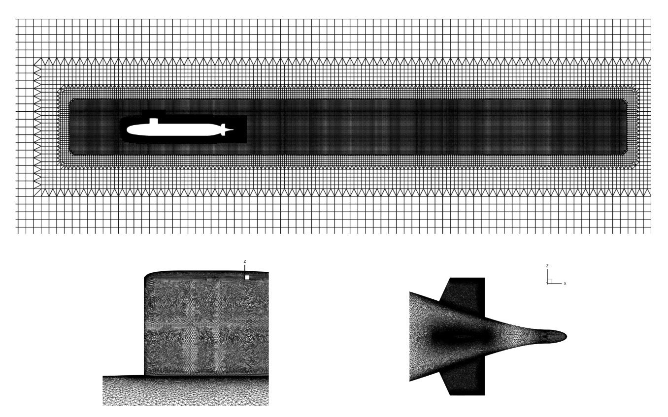
Fig. 5.13.2 Overview of surface and volume mesh (higher resolution).

Simulation Parameters

To replicate the experimental setup and eliminate boundary-induced disturbances in the flow, an automated far-field boundary was generated, extending 100 times the ship’s length between perpendiculars in all directions. This generously sized domain ensures that pressure waves, vortices, and other flow features generated by the submarine do not reflect off the boundaries and interfere with the solution. Maintaining this distance minimizes artificial interactions and helps reproduce the ideal free-stream conditions observed during the experiments.

The model was analyzed at the same speeds used in the original experimental campaign. The tested freestream velocities, expressed in knots, were:

(5.13.1)\[\mathbf{V} = [5.93,\ 10.00,\ 11.85,\ 13.92,\ 16.00,\ 17.79]\ \text{knots}\]

The solver was configured for optimal performance in low-Mach-number, incompressible flow regimes. Flow360’s compressible solver settings were carefully adjusted to operate efficiently under these conditions, with particular attention given to convergence criteria and numerical schemes appropriate for low-speed flows. The freestream fluid properties were matched to the experimental conditions to ensure consistency. A no-slip wall boundary condition was applied to all submarine surfaces to accurately represent the physical interaction between the fluid and geometry, which is critical for resolving boundary layer development and capturing shear forces that contribute to hydrodynamic resistance.

Table 5.13.2 Simulation Parameters

Section	Parameter	Value	Units
Geometry	Reference area	6.349	m²
Operating Condition	Medium	Liquid	—
	Velocity magnitude	Case dependent	knot
	Reference velocity magnitude	Case dependent	knot
	Density	1000	kg/m³
	Dynamic viscosity	0.001002	kg/(m·s)
	Turbulent Viscosity Ratio	10	—
Flow solver	Mode	Steady	—
	Max steps	5000	—
	CFL type	Adaptive CFL	—
Turbulence Model	Model	Spalart-Allmaras	—
	Absolute tolerance	1e-8	—
Navier-Stokes Solver	Absolute tolerance	1e-10	—
	Kappa MUSCL	-0.33	—
	Low Mach preconditioner	True	—

After completing the steady-state simulations, additional Delayed Detached Eddy Simulations (DDES) were performed to obtain time-accurate solutions. The results from the preceding RANS cases were used as initial conditions for the DDES runs via the fork function. DDES inherently captures more detailed aspects of fluid behavior by directly resolving turbulence in the wake of the submarine. This results in improved accuracy in both pressure distribution predictions and overall flow field modeling. The additional parameters used are summarized below:

Table 5.13.3 Time Accurate Simulation Parameters

Section	Parameter	Value
Flow solver	Mode	Unsteady
	Steps	5000
	Step Size	5e-5s
	Max pseudo steps	50
Turbulence Model	Model	Spalart-Allmaras
	Relative tolerance	1e-2
	Hybrid Model	DDES
	Grid Size for LES	Max Edge Length
Navier-Stokes Solver	Relative tolerance	1e-2

Results and Validation

To benchmark the performance of Flow360 in tackling incompressible simulations, the submarine’s performance was evaluated across a range of velocities, mirroring the conditions of the original experimental case study. This systematic approach allows for the assessment of Flow360’s predictive capability across varying Reynolds numbers, which is essential in understanding its robustness and accuracy when modeling underwater hydrodynamics.

The results have been analyzed both in terms of the total resistance generated against the submarine’s forward motion and through detailed visualizations of the flow fields. All results such as resistance predictions, velocity flow-fields, and surface shear stress and pressure distributions, have been validated against the publicly available experimental data.

This combined assessment offers a practical and intuitive means of verifying that the simulated flow adheres to expected hydrodynamic behavior, such as boundary layer development, wake formation, and flow separation regions. Therefore, validating the solver’s capability to replicate key physical phenomena governing underwater vehicle performance.

Mesh Sensitivity Study

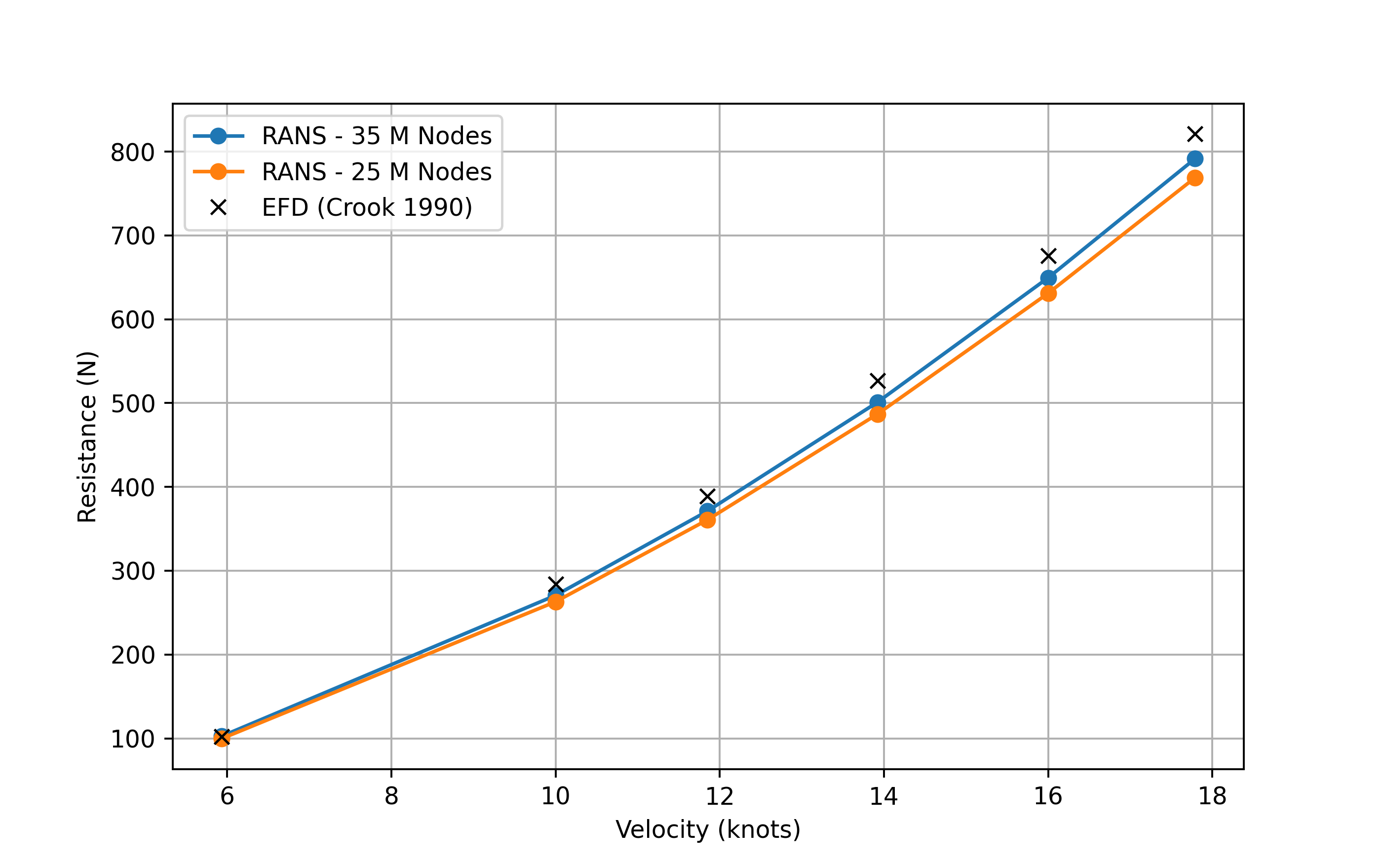
Fig. 5.13.3 Mesh Sensitivity study.

A mesh sensitivity study has been carried out to ensure that the simulation results are independent of mesh resolution. To this end, we have compared resistance predictions obtained using the two mesh configurations described in the previous section. The comparison revealed an improvement of approximately 2% in prediction accuracy when using the finer mesh. The small differences between the different meshes confirms that no further refinement is needed.

Resistance Prediction Analysis

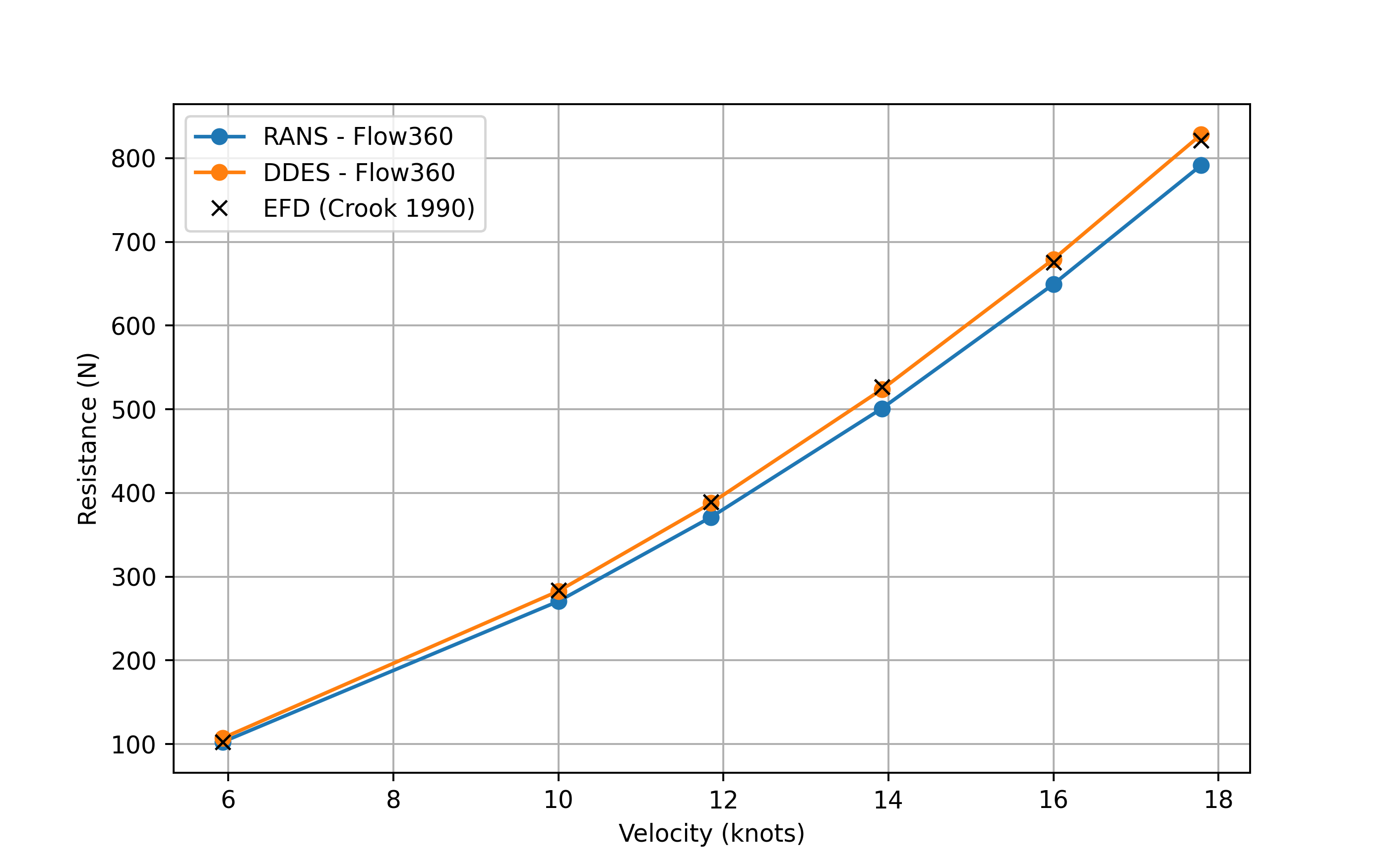
Fig. 5.13.4 Predicted resistance comparison of Suboff Model.

The data obtained through Reynolds-Averaged Navier–Stokes (RANS) simulations closely matches the experimental results. Analyzing the predicted resistance, Flow360, is able to provide an accuracy of around 4% across the whole range of working speeds.At the most heavily validated speed of 5.93 knots, the error is of less than 2%.

The DDES simulations demonstrate significantly higher accuracy, yielding an error of less than 1% in all cases except the first, where the deviation is limited to 5 N. This improved performance can be attributed to DDES’s capability to resolve large-scale turbulent structures, which, in this case, play a critical role in the accuracy of the resistance prediction. These results serve to validate both Flow360 and its turbulence modeling approach, confirming their ability to deliver high-fidelity simulations beyond conventional RANS accuracy levels.

Table 5.13.4 Resistance Prediction Errors using DDES

Velocity (knots)	Error (N)	Error (%)
5.93	-4.82	4.70
10.0	1.03	-0.36
11.85	1.35	-0.34
13.92	2.84	-0.53
16.0	-3.74	0.55
17.79	-7.17	0.87
Absolute Error Mean	3.5	1.23

Overall, the solver demonstrates the capability to accurately predict the estimated drag within a 0.5-knot margin of vehicle speed when using time-averaged simulations, and with near-exact agreement when employing time-accurate analysis.

Surface Pressure and Skin Friction Coefficients

Experimental data on surface coefficients is only available for the lowest velocity case. Therefore, this section focuses exclusively on that condition. Both the numerical and experimental data were collected along the submarine’s vertical symmetry plane.

Surface Pressure Distribution	Surface Friction Distribution
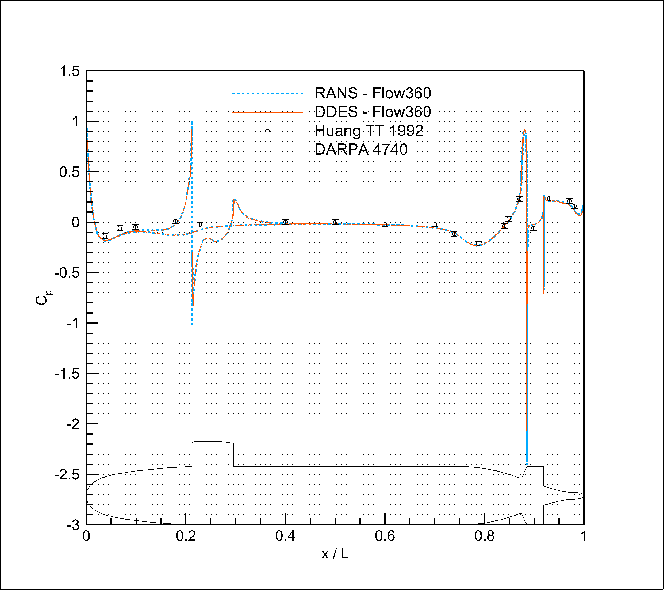
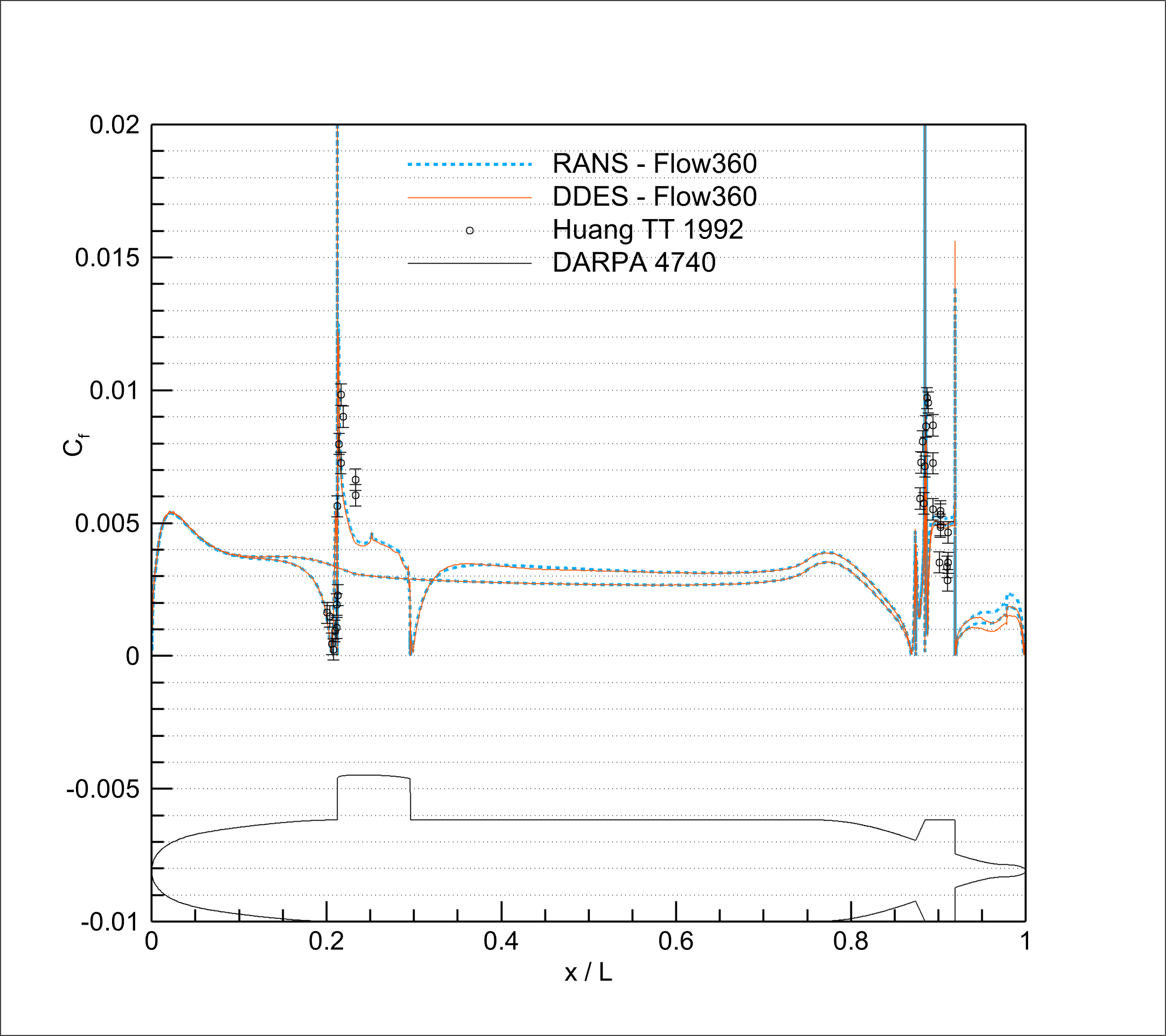
Fig. 5.13.5–5.13.6 Surface distributions.

The predicted surface pressure coefficients show excellent agreement with the experimental data, highlighting the software’s capability to accurately model boundary layer behavior along the length of the submarine. Notably, distinct peaks appear in critical regions such as the sail and stern, where flow acceleration and deceleration are most pronounced. This demonstrates Flow360’s ability to resolve complex flow features in areas characterized by strong curvature, flow separation, and reattachment, key challenges in hydrodynamic simulations.

DDES and RANS results seems to show little difference in terms of surface distributions. This result is expected as the overall results are similar in both cases. It is important to note that, even small changes in surface pressure distributions can lead to significant overall drag differences when integrating the pressure field along the surface of the ship, as happens in this case.

Radially Averaged Streamwise Velocity Field

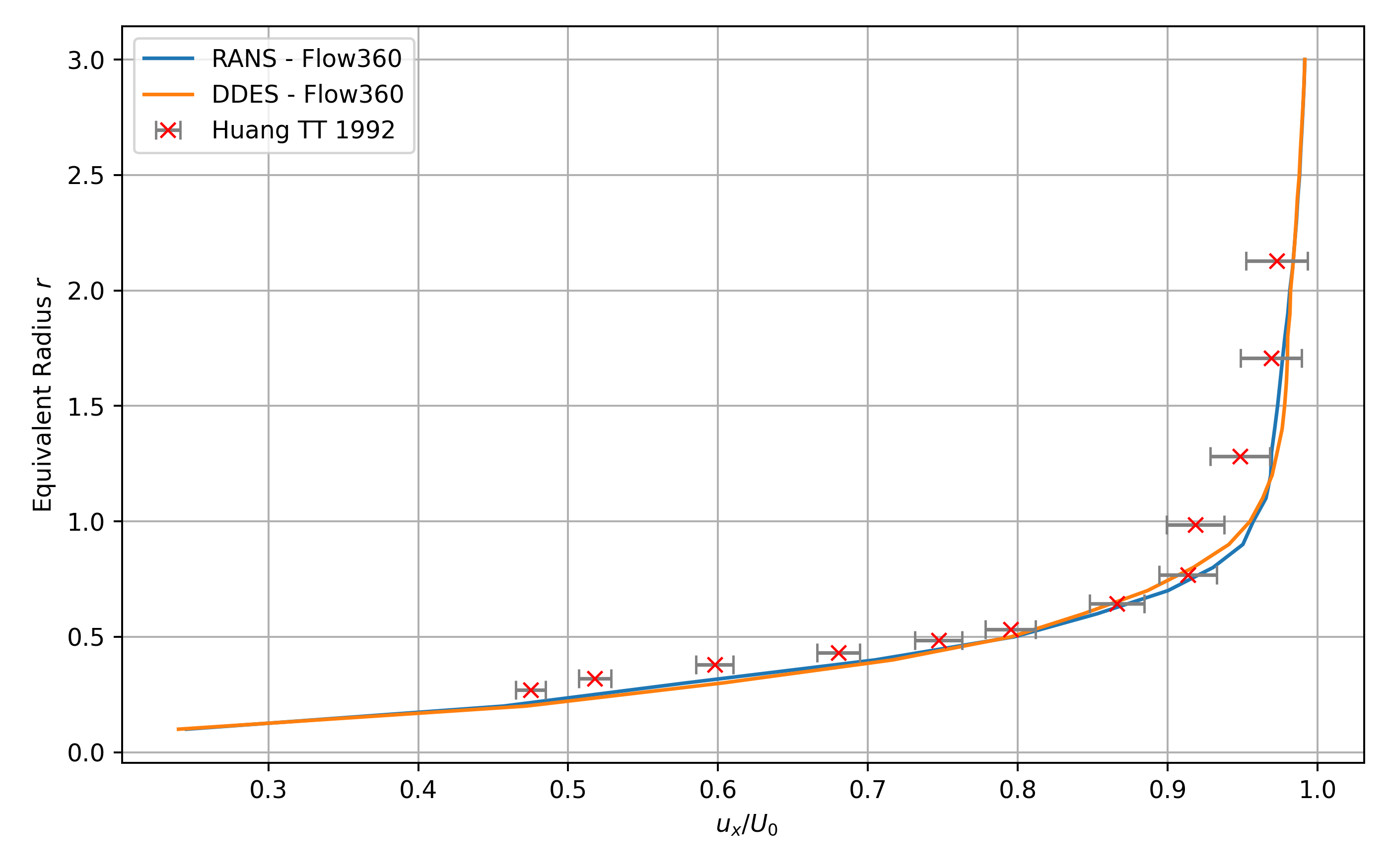
Fig. 5.13.5 Mean streamwise velocity prediction compared with experimental data.

The normalized streamwise velocity component is analyzed as a function of a normalized radius, defined as the radial distance from the hull’s symmetry axis divided by the radius at the midship section. These results correspond to measurements taken at the propeller plane, which is located at 0.978 \(L\) along the x-axis and oriented perpendicular to it, where \(L\) is the length between perpendiculars.

As happened for surface coefficients, velocity flowfield analysis was experimentally only carried out at 5.93 knots.

The numerical results show strong agreement with the flowfield visualizations reported by Huang et al. [2]. The experimental data is presented with associated error bars of 2.1%.

The numerical results slightly underpredict the velocity magnitude near the centerline, at smaller normalized radii, but exhibit excellent agreement at larger radii, farther from the hull axis. This trend is observed consistently in both RANS and DDES simulations. Overall, the numerical model successfully captures the increase in velocity with radial distance, closely matching the experimentally observed trend.

Conclusion

This validation study demonstrates Flow360’s ability to accurately simulate incompressible flows around submerged geometries, using the DARPA SUBOFF Model 4740 as a benchmark. The solver successfully captures key hydrodynamic features observed in experiments, including surface pressure and skin-friction distributions, total resistance trends and velocity patterns near the propeller plane. Resistance predictions show errors below 4% for time-averaged simulations and as low as 1.23% for time-accurate simulations. Local flow quantities are also captured with the same accuracy, highlighting the solver’s robustness and reliability for underwater applications. These results confirm that Flow360 is well-suited for high-fidelity modeling of submarine performance and other marine systems in incompressible flow regimes.

References

[1] (1,2)

Roddy, R. F., Investigation of the Stability and Control Characteristics of Several Configurations of the DARPA SUBOFF Model (DTRC Model 5470) from Captive-Model Experiments, Departmental Report DTRC/SHD-1298-08, David Taylor Research Center, Bethesda, MD, 1990. Available online

[2] (1,2)

Huang TT, Liu H-L, Groves NC, Forlini TJ, Blanton J, Gowing S. Measurements of flows over an axisymmetric body with various appendages (DARPA SUBOFF Experiments). In: 19th Symp. on naval hydrodynamics, Seoul, Korea; 1992. Available online