7.10. User Defined Dynamics

In Flow360, users are able to specify arbitrary dynamics. This section provides an example for a Proportional-Integral (PI) controller and an example for Aero-Structural Interaction (ASI).

7.10.1. PI Controller for Angle of Attack to Control Lift Coefficient

In this example, we add a controller to the om6Wing case study. Based on the entries of the configuration file in this case study, the resulting value of the lift coefficient, CL, obtained from the simulation is ~0.26. Our objective is to add a controller to this case study such that for a given target value of CL (e.g., 0.4), the required angle of attack, alphaAngle , is estimated. To this end, a PI controller is defined under userDefinedDynamics in the configuration file as:

"userDefinedDynamics": [
    {
        "dynamicsName": "alphaController",
        "inputVars": [
            "CL"
        ],
        "constants": {
            "CLTarget": 0.4,
            "Kp": 0.2,
            "Ki": 0.002
        },
        "outputVars": {
            "alphaAngle": "if (pseudoStep > 500) state[0]; else alphaAngle;"
        },
        "stateVarsInitialValue": [
            "alphaAngle",
            "0.0"
        ],
        "updateLaw": [
            "if (pseudoStep > 500) state[0] + Kp * (CLTarget - CL) + Ki * state[1]; else state[0];",
            "if (pseudoStep > 500) state[1] + (CLTarget - CL); else state[1];"
        ],
        "inputBoundaryPatches": [
            "1"
        ]
    }
]

More details for some of the parameters are explained below:

1. dynamicsName: This is a name given by the user for the dynamics. The results of user-defined dynamics are saved to “udd_dynamicsName_v2.csv”.

2. constants: This includes a list of all the constants related to this UDD. These constants will be used in the equations for updateLaw and outputVars. In the above-mentioned example, CLTarget, Kp, and Ki are the target value of the lift coefficient, the proportional gain of the controller, and the integral gain of the controller, respectively.

3. outputVars: Each outputVars consists of the variable name and the relations between the variable and the state variables. For this example, we set the output variable equal to the angle of attack calculated by the controller after the first 500 pseudoSteps (i.e., state[0]).

4. stateVarsInitialValue: There are two state variables for this controller. The first one, state[0], is the angle of attack computed by the controller, and the second one, state[1], is the summation of error (CLTarget - CL) over iterations. The initial values of state[0] and state[1] are set to alphaAngle and 0, respectively.

The equation for the control system can be thus written as:

(7.10.1)\[ \begin{align}\begin{aligned}\alpha^n = \alpha^{n-1} + \left[ K_p \cdot (C_{L,target} - C_L^n) + K_i \cdot e^n \right]\\e^n = e^{n-1} + C_{L,target} - C_L^n\end{aligned}\end{align} \]

where the superscript \(n\) denotes pseudo step, alphaAngle (\(\alpha\)) is state[0] and the integral of error (\(e\)) is state[1].

5. updateLaw: The expressions for the state variables are specified here. The first and the second expressions correspond to equations for state[0] and state[1], respectively. The conditional statement forces the controller to not be run for the first 500 pseudoSteps. This ensures that the flow field is established before the controller is initialized.

6. inputBoundaryPatches: The related boundary conditions for the inputs of the user-defined dynamics are specified here. In this example, the noSlipWall boundary conditions are where CL is calculated. As seen in the configuration file, the boundary name for the No-Slip boundary condition is "1".

The following figure shows the values of lift coefficient, CL, and angle of attack, alphaAngle, versus the steps, pseudoStep. As specified in the configuration file, the initial value of angle of attack is 3.06. With the specified user-defined dynamics, alphaAngle is adjusted to a final value of 4.61 so that CL = 0.4 is achieved.

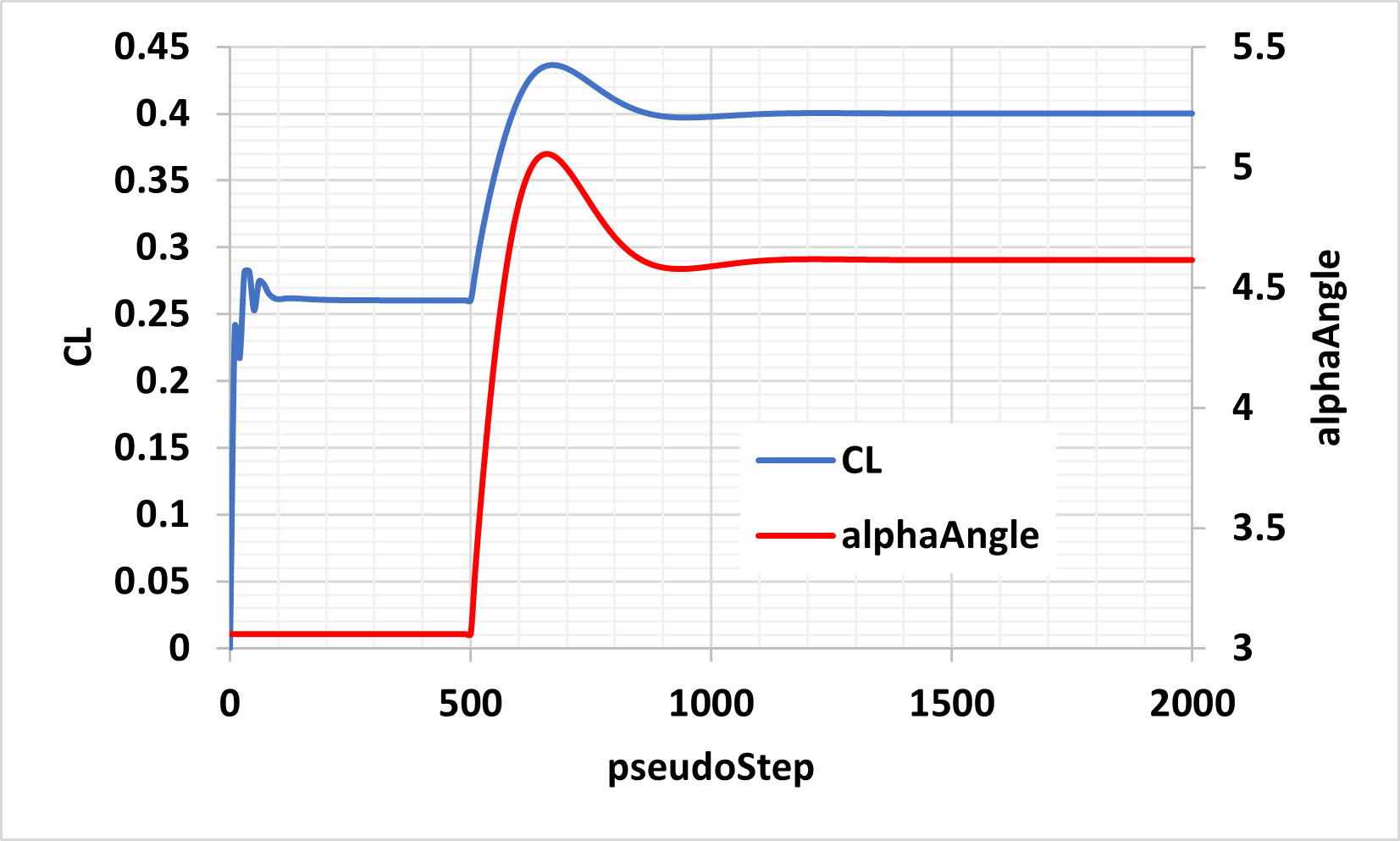
Fig. 7.10.1 Results of alphaController for om6Wing case study.

7.10.2. Dynamic Grid Rotation using Structural Aerodynamic Load

In this example, we present an illustrative case where a flat plate rotates while being subjected to a rotational spring moment and damper as well as aerodynamic loads.

As you can see below, the flate plate mesh consists of two zones separated by a circular sliding interface. The inner zone will rotate while the outer zone remains stationary. This is the same mesh topology as what is used for rotating propeller simulations.

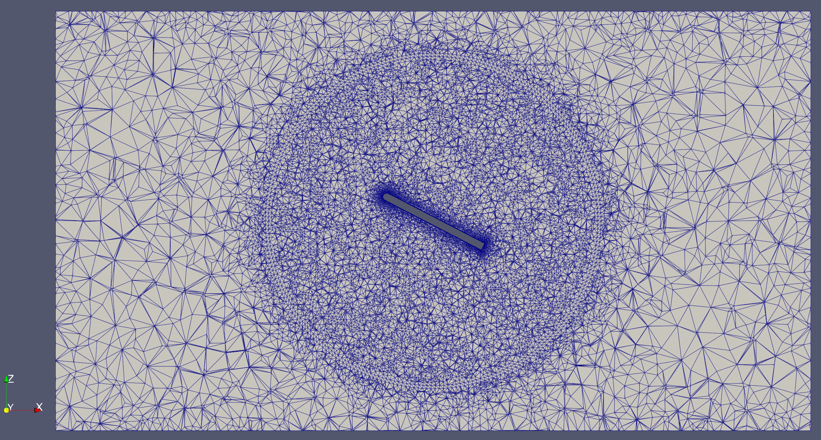
Fig. 7.10.2 Mesh of flat plate showing sliding interface for rotation.

Below is a video showing the flutter motion of the plate.

Fig. 7.10.3 Flutter motion of the plate under aerodynamic and structural forces.

The userDefinedDynamics and slidingInterfaces section of the case JSON is presented below:

{
    "slidingInterfaces": [
        {
            "stationaryPatches": [
                "farFieldBlock/rotIntf"
            ],
            "rotatingPatches": [
                "plateBlock/rotIntf"
            ],
            "axisOfRotation": [
                0,
                1,
                0
            ],
            "centerOfRotation": [
                0,
                0,
                0
            ],
            "volumeName": "plateBlock",
            "theta": [
                "0",
                "0",
                "0"
            ]
        }
    ],
    "userDefinedDynamics": [
        {
            "dynamicsName": "dynamicTheta",
            "inputVars": [
                "momentY"
            ],
            "constants": {
                "I": 0.443768309310345,
                "zeta": 4.0,
                "K": 0.0161227107,
                "omegaN": 0.190607889,
                "theta0": 0.0872664626
            },
            "outputVars": {
                "omegaDot": "state[0];",
                "omega": "state[1];",
                "theta": "state[2];"
            },
            "stateVarsInitialValue": [
                "-1.82621384e-02",
                "0.0",
                "1.39626340e-01"
            ],
            "updateLaw": [
                "if (pseudoStep == 0) (momentY - K * ( state[2] - theta0 ) - 2 * zeta * omegaN * I *state[1] ) / I; else state[0];",
                "if (pseudoStep == 0) state[1] + state[0] * timeStepSize; else state[1];",
                "if (pseudoStep == 0) state[2] + state[1] * timeStepSize; else state[2];"
            ],
            "inputBoundaryPatches": [
                "plateBlock/noSlipWall"
            ],
            "outputTargetName": "plateBlock"
        }
    ]
}

For this case the dynamics of the plate are:

(7.10.2)\[ \begin{align}\begin{aligned}\dot{\omega} = \left[ \tau_y - K \cdot \left( \theta-\theta_0 \right) - 2\zeta\omega_N I \omega \right]/I\\ \omega -\omega_0= \int_{0}^{t} \dot{\omega}\left(t'\right) \, dt'\\ \theta -\theta_0 = \int_{0}^{t} \omega\left(t'\right) \, dt'\end{aligned}\end{align} \]

which corresponds to the three updateLaw arguments in the above JSON input file. The symbols are defined in the table below.

Symbol	Description
\(\theta\)	Rotation angle of the plate in radians.
\(\omega\)	Rotation velocity of the plate in radians.
\(\dot{\omega}\)	Rotation acceleration of the plate in radians.
\(\tau_y\)	Aerodynamic moment exerted on the plate.
\(K\)	Stiffness of the spring attached to the plate at the structural support.
\(\zeta\)	Structural damping ratio.
\(\omega_N\)	Structural natural angular frequency.
\(I\)	Structural moment of inertia.

In the inputVars, the momentY is the y-component of the rotational moment imposed by the aerodynamic loading. The moment is calculated relative to the momentCenter on "plateBlock/noSlipWall".

The name of rotating volume zone that we want to control is plateBlock and thus the "outputTargetName" is set to plateBlock. The first, second and third state variable correspond to \(\dot{\omega}\), \(\omega\), and \(\theta\), respectively.

7.10.3. Custom set of user defined forces and moments

In this example we will use a simple airplane geometry with control surfaces (aileron and rudders) to showcase how a user could calculate user defined forces and moments to track the evolution of the torque on the control surfaces as the simulation converges.

To generate the geometry and associated mesh we will simply use these input csm , mesh surface definition , volume definition. See this example tutorial or this one for more information on how to do that.

As you can see in this image below, the airplane has 2 ailerons and 2 rudders. All 4 control surfaces move in a simple rotation around an axis. For each of these we will monitor the torque around the rotation axis.

Note

Due to the coarseness of the mesh settings selected, the solver may give you a warning when you go to submit the case with that configuration. You can ignore it and proceed to the case submission.

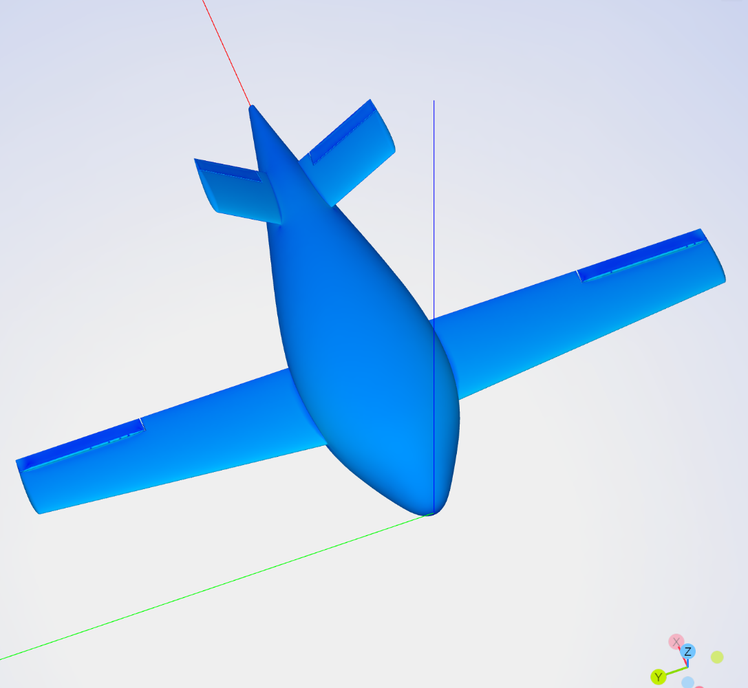
Fig. 7.10.4 Isometric view of a simple airplane with 4 control surfaces

Now that we have a volume mesh ready we need to define the run parameters. In this tutorial we will focus on the definition of userDefinedDynamics. Please download this sample input json file. The setup is for our simple airplane flying at 50m/s at 10 ° angle of attack.

The control surfaces have their rotation centers and axes as:

Name	rotation Center	rotation Axis
right Aileron	(5.7542, 7, 0)	(0, 1, 0)
left Aileron	(5.7542, -7, 0)	(0, -1, 0)
right Rudder	(12.01, 0.861, 0.861)	(0, 0.7071, 0.7071)
left Rudder	(12.01, -0.861, 0.861)	(0, -0.7071, 0.7071)

Note

In this tutorial we have arbitrarily set the geometry/momentCenter at the same X and Z location as the Aileron rotation axes ( as in, on the Ailerons’ rotation axes). Since the aileron hinges axes is aligned with the Y axis, this allows us to check the hinge moment values we get for the ailerons against the Moment Y value for that same aileron automatically generated by the software. They are the same.

The interesting part is the definition of the control surface hinge moments via user defined variables and the automatic tracking of the outputs to get the evolution of those forces as the run converges to see if we have reached satisfactory convergence of the desired forces and moments.

Here, we will convert the monitored torques into SI forces (N) and moments (Nm).

The input json file has an optional userDefinedDynamics (UDD) section which contains 4 similar items. Each control surface requires its own userDefinedDynamics instance with the only differences being the names and geometric inputs for each control surface as per the table above.

If we look at the “userDefinedDynamics” section of the configuration json file we see that the UDD instance has 4 items each containing 6 sections. The 4 items are the 4 control surfaces. The 6 sections are described below.

Fig. 7.10.5 UDD section of the case configuration json file.

7.10.3.1. constants

Named constants that will be used in the update law. “newCenterX,Y,Z” and “newAxisX,Y,Z” are the coordinates of the new moment reference center and rotation axes we want to project onto. They define the aileron or rudder’s hingelines.

"constants": {
    "density_kgpm3": 1.225,
    "c_inf_mps": 340.2,
    "l_grid_unit": 1,
    "newCenterX": 5.7542,
    "newCenterY": 7,
    "newCenterZ": 0,
    "newAxisX": 0,
    "newAxisY": 1,
    "newAxisZ": 0
}

7.10.3.2. updateLaw

This block is a list of expressions used to define the outputs we want to save. Because we convert the raw solver outputs to dimensional metric value we need to calculate the \(\rho_\infty C_\infty^2 L_\text{gridUnit}^3\) :ref:` moment dimensionalization values<nondim_output>`.

The equation on lines 2 defines that dimensionalization value. Lines 3 to 5 define the new dimensional moments as per the new moment reference center and rotation axis we defined above. The last line defines the total hinge moment, as in the torque that the control surface’s actuating mechanism will have to overcome to rotate the control surface.

"updateLaw": [
    "density_kgpm3 * c_inf_mps * c_inf_mps * l_grid_unit * l_grid_unit * l_grid_unit",
    "(rotMomentX - ((newCenterY - momentCenterY) * forceZ - (newCenterZ - momentCenterZ) * forceY)) * state [0];",
    "(rotMomentY + ((newCenterX - momentCenterX) * forceZ - (newCenterZ - momentCenterZ) * forceX)) * state [0];",
    "(rotMomentZ - ((newCenterX - momentCenterX) * forceY - (newCenterY - momentCenterY) * forceX)) * state [0];",
    "state[1] * newAxisX + state[2] * newAxisY + state[3] * newAxisZ "
]

7.10.3.3. inputBoundaryPatches

Patches of the mesh that we want to apply the calculations to. For example:

"inputBoundaryPatches": [ "fluid/aileronRight" ]

7.10.3.4. visualizing the results

All the UDD outputs can be downloaded in the results/udd_DYNAMICSNAME_v2.csv where DYNAMICSNAME matches the values entered in the “dynamicsName” section.

They can also be automatically visualized in the Monitors tab for that case on our website. Remember that the hinge torque’s dimensional value is calculated in state[4]. By clicking on each line’s legend icon you can disable the values you are not interested in, leaving only the desired values’ convergence history displayed.

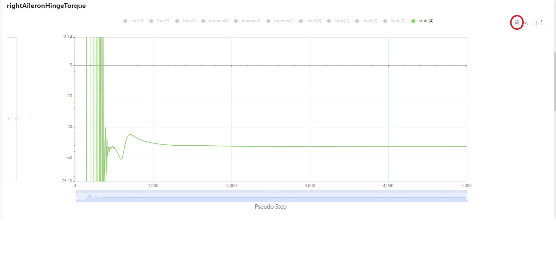
Fig. 7.10.6 Dimensional hinge torque convergence history for the right Aileron.

A good way to check that the calculations are correct is to compare the overall forces on a given component with the resulting torque values. If you recall above it was mentioned that we have purposefully put the simulation geometry/momentCenter on the aileron hinge line. Both are at X=5.7542 and since the aileron hinge vector [0,1,0] is aligned with the Y axis, the left and right aileron My magnitudes are identical to the left and right aileron hinge torque. The left aileron has it hinge vector set to [0,-1,0] hence the sign will be flipped between My and hinge torque.

To check that the calculations are correct let’s get the final value of the right aileron hinge torque. To do that please click on the DataView icon circled in red in the above figure. Scroll to the state[4] column and down to the last row. Make sure to navigate to the table’s final section(by clicking on the 6 below the table as circled in red below) That highlighted value of -52.65Nm is the right aileron hinge torque in dimensional Newton-meters.

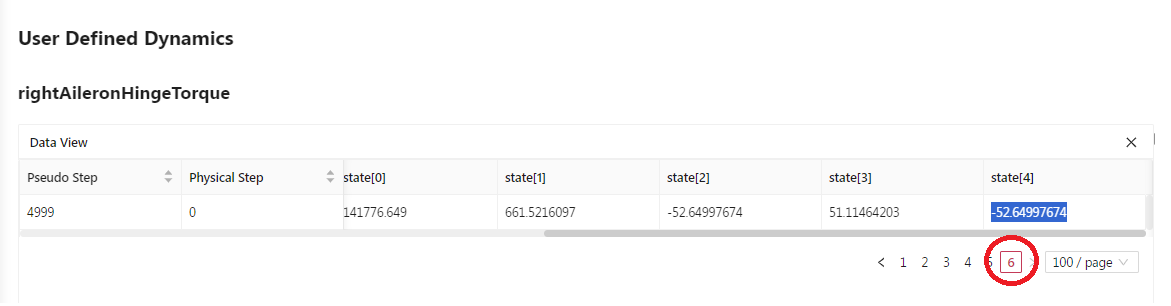
Fig. 7.10.7 Dimensional hinge torque table for the right Aileron.

Now by going back to the Forces tab, down to the Forces and Moments by surface section, we can similarly find the final CMy= \(-5.73 \times 10^{-4}\) for the right aileron:

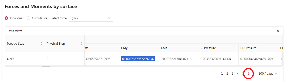
Fig. 7.10.8 CMy table for the right Aileron.

Now if we dimensionalize that value, we get

(7.10.3)\[\begin{split}\begin{align} -5.73 \times 10^{-4} &\cdot \frac{1}{2} \rho_\infty U_\text{ref}^2 A_\text{ref} L_\text{ref}\left[1\right] \\ &= -5.73\times 10^{-4} \cdot \frac{1}{2} \cdot 1.225\frac{kg}{m^3} \cdot (50\frac{m}{s})^2 \cdot 60m^2 \cdot 1m \\ &= -52.65N \cdot m \end{align}\end{split}\]