7.3. Time-accurate RANS CFD on a propeller using a sliding interface: the XV-15 rotor geometry

The XV-15 tiltotor aircraft is a commonly used test bed for propeller validation work. As you can see from the following papers, we have done extensive validation work on this geometry. We will now use it to show you how to analyze a propeller-type geometry using a sliding mesh interface.

• Rotor5: Rotor analysis under 5 hours using ultra-fast and high-fidelity CFD simulation and automatic meshing

• Assessment of Detached Eddy Simulation and Sliding Mesh Interface in Predicting Tiltrotor Performance in Helicopter and Airplane Modes

This same geometry and case was already used in a Quick Start example. Here we will go more in depth into how to get a sliding interface case setup.

Rotational and stationary volumes

In order to run a rotating geometry we need to set up a mesh with two blocks, an inner “rotational volume” and an outer “stationary volume”. The interface between those two volumes needs to be a solid of revolution (i.e., sphere, cylinder, etc.).

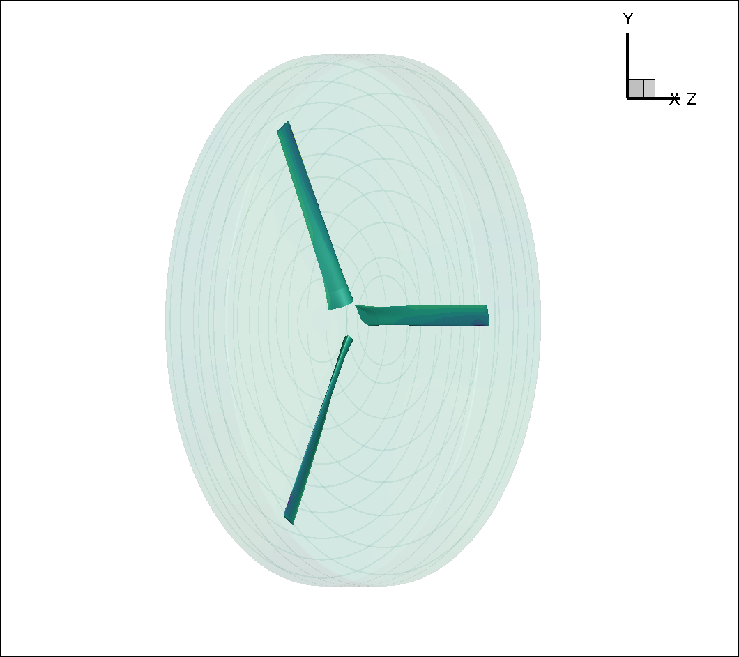
Fig. 7.3.1 Inner block enclosing the XV-15 3-bladed prop

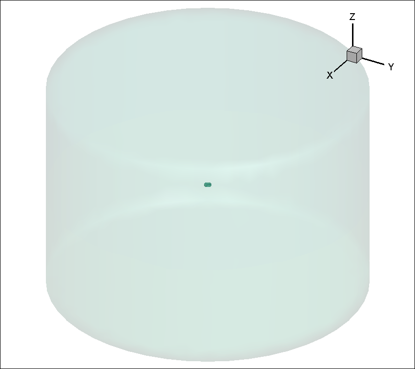
Fig. 7.3.2 Farfield volume enclosing inner block

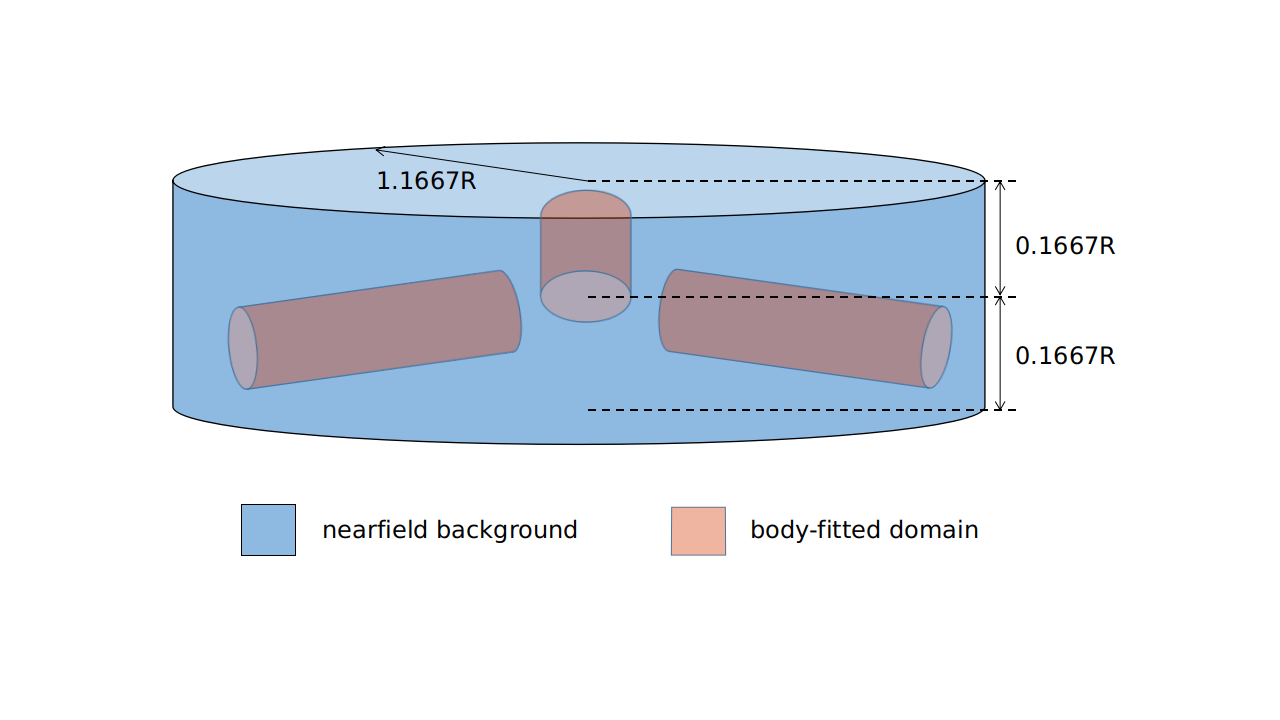
Fig. 7.3.3 Body-fitted cylinder blocks inside a larger nearfield domain

Please note that it is possible, just like in the figure above, to set up nested sliding interfaces to simulate, for example, a rotating propeller with blades that pitch as they rotate (i.e., a helicopter's cyclical). We could also put many rotating blocks inside the stationary farfield block to simulate multiple rotors.

Sliding interface requirements

Added in version release-23.3.2.0: Starting from release 23.3.2.0 of flow360, sliding interfaces no longer need to be constructed with concentric rings. Instead, they can be made of any unstructured mesh that includes triangular and/or quadrilateral elements. Please see the mesh sliding interface entry

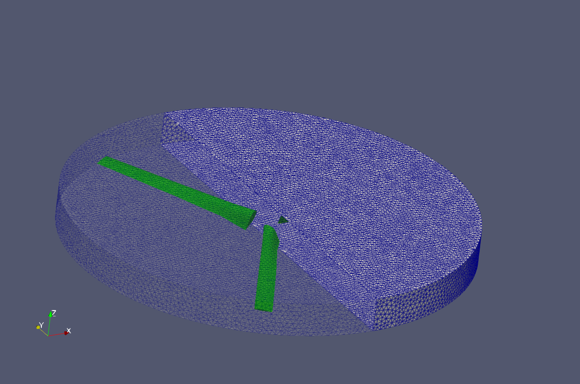
Fig. 7.3.4 Arbitrarily unstructured sliding interface mesh. (Half of the interface is made transluscent to show the enclosed blades)

XV-15 setup

The rotor has a 150” (inches) radius and the blades have a chord of roughly 11”. For simplicity’s sake we will use the SI system and convert these to 3.81 m radius and 0.279 m chord.

A complete CGNS mesh is available here.

Attention

The mesh file must be in the CGNS format if it contains multiple volume zones.

The XV15_Hover_ascent_coarse_v2.cgns mesh contains the following blocks and associated boundaries and zone grid connectivities. See CGNS Knowledge Base for more details .

farField
    <Boundaries>:
        farField
    <ZoneGridConnectivity>:
        innerRotating
innerRotating
    <Boundaries>:
        blade
    <ZoneGridConnectivity>:
        farField

This shows us that we have two volume mesh zones (farField and innerRotating). Inside innerRotating we have the blade NoSlipWall boundary. Associated with the farField zone is the farField boundary. Each zone also has information about zone grid connectivity, which tells Flow360 that innerRotating and farField volume zones are adjacent to each other.

Uploading your mesh

With the mesh file and its associated mesh configuration json file. You can upload the mesh either by using the Web UI or the Python API.

Defining a case using Flow360 Python API.

Once your mesh has been uploaded, the last step before launching a run is to create a python script with all the information needed by Flow360 to run your case. Here a sample Python Script is provided. Please refer to the Python API Guide and Reference sections for details about how to create the python script.

Case input conditions

For our case we have the following operating conditions:

• Airspeed = 5 m/s

• Rotation rate = 600 RPM

• Speed of sound = 340.2 m/s

• Density = 1.225 kg/m³

• Alpha = -90 °, air coming down from above (i.e., an ascent case)

Other key considerations:

• The reference velocity magnitude is arbitrarily set to the tip velocity magnitude of the blades, with an estimated \(\text{Mach} \approx 0.7\) (238.14 m/s)

• For simulation, we will do 5 revolutions at 3 ° per time step, thus 600 physical time steps in total

We use the Flow360 Python API to set up the rotation zone, operating condition, time stepping, volume and surface models as follows:

rotation_zone = volume_mesh["innerRotating"]
rotation_zone.center = (0, 0, 0) * fl.u.m
rotation_zone.axis = (0, 0, -1)
operating_condition=fl.AerospaceCondition(
    velocity_magnitude=5 * fl.u.m / fl.u.s,
    alpha=-90 * fl.u.deg,
    reference_velocity_magnitude=238.14 * fl.u.m / fl.u.s,
)
time_stepping=fl.Unsteady(
    max_pseudo_steps=35,
    steps=600,
    step_size=0.5 / 600 * fl.u.s,
    CFL=fl.AdaptiveCFL(),
)
models=[
    fl.Fluid(
        navier_stokes_solver=fl.NavierStokesSolver(
            absolute_tolerance=1e-9,
            linear_solver=fl.LinearSolver(max_iterations=35),
        ),
        turbulence_model_solver=fl.SpalartAllmaras(
            absolute_tolerance=1e-8,
            linear_solver=fl.LinearSolver(max_iterations=25),
            DDES=True,
            rotation_correction=True,
            equation_evaluation_frequency=1,
        ),
    ),
    fl.Rotation(
        volumes=rotation_zone,
        spec=fl.AngularVelocity(600 * fl.u.rpm),
    ),
    fl.Freestream(surfaces=volume_mesh["farField/farField"], name="Freestream"),
    fl.Wall(surfaces=volume_mesh["innerRotating/blade"], name="NoSlipWall"),
]

Case running

As mentioned in the Quick Start example, using either the Web UI or the Python API please launch a new case using the mesh you have uploaded above and the python script you have just downloaded. The simulation takes about 3.5 to 4 minutes to run 5 revolutions.

For a time accurate case to be considered well converged we like to have at least 2 orders of magnitude in the residuals within each time step.

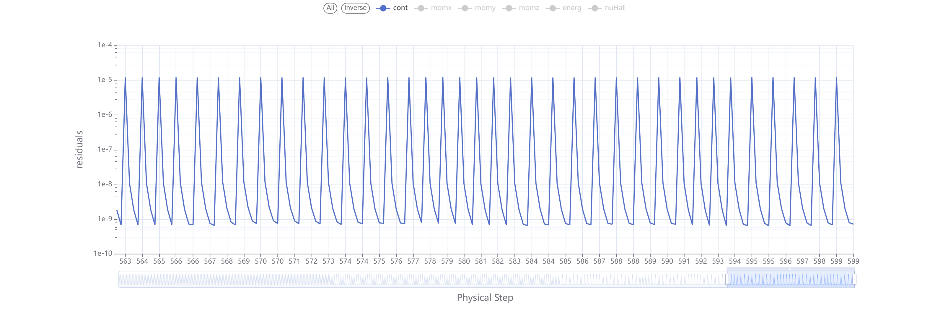
Fig. 7.3.5 Convergence plot showing more then 2 orders of magnitude decrease in the residuals for each time step.

The forces also seem to have stabilized after running for 5 revolutions.

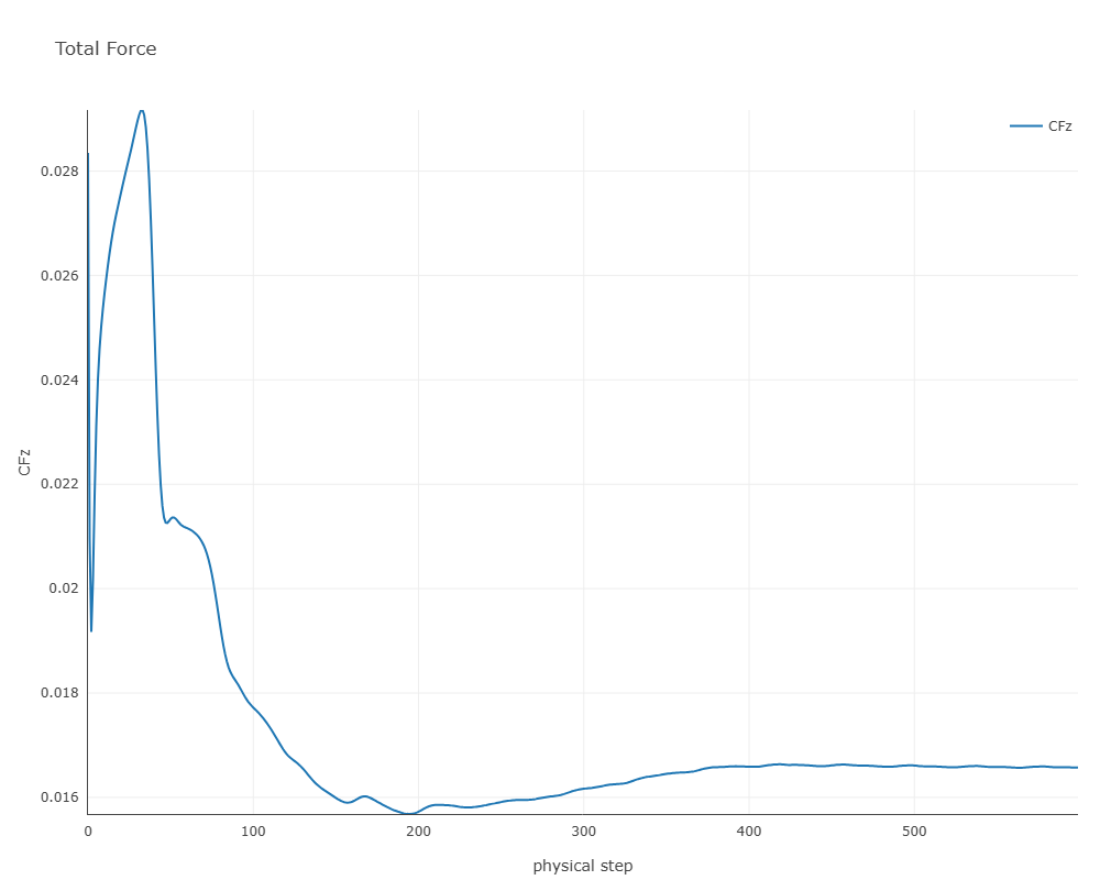
Fig. 7.3.6 Force history plot showing good stabilization of the forces.

Congratulations. You have now run your first propeller using a sliding interface in Flow360.