Running the quickstart via the API

Flow360 can be automatically driven via our powerful Python API. All the case setup parameters available in the WebUI are available in the Python API.

By starting from the same evtol_quickstart_grouped.csm file as we have downloaded in the above geometry upload section, The EVTOL quickstart case shown previously can be easily launched using the following code:

# Import necessary modules from the Flow360 library
from matplotlib.pyplot import show

import flow360 as fl
from flow360.examples import Airplane

# Step 1: Create a new project from a predefined geometry file in the Airplane example
# This initializes a project with the specified geometry and assigns it a name.
project = fl.Project.from_geometry(
    Airplane.geometry,
    name="Python Project (Geometry, from file)",
)
geo = project.geometry  # Access the geometry of the project

# Step 2: Display available groupings in the geometry (helpful for identifying group names)
geo.show_available_groupings(verbose_mode=True)

# Step 3: Group faces by a specific tag for easier reference in defining `Surface` objects
geo.group_faces_by_tag("groupName")

# Step 4: Define simulation parameters within a specific unit system
with fl.SI_unit_system:
    # Define an automated far-field boundary condition for the simulation
    far_field_zone = fl.AutomatedFarfield()

    # Set up the main simulation parameters
    params = fl.SimulationParams(
        # Meshing parameters, including boundary layer and maximum edge length
        meshing=fl.MeshingParams(
            defaults=fl.MeshingDefaults(
                boundary_layer_first_layer_thickness=0.001,  # Boundary layer thickness
                surface_max_edge_length=1,  # Maximum edge length on surfaces
            ),
            volume_zones=[far_field_zone],  # Apply the automated far-field boundary condition
        ),
        # Reference geometry parameters for the simulation (e.g., center of pressure)
        reference_geometry=fl.ReferenceGeometry(),
        # Operating conditions: setting speed and angle of attack for the simulation
        operating_condition=fl.AerospaceCondition(
            velocity_magnitude=100,  # Velocity of 100 m/s
            alpha=5 * fl.u.deg,  # Angle of attack of 5 degrees
        ),
        # Time-stepping configuration: specifying steady-state with a maximum step limit
        time_stepping=fl.Steady(max_steps=1000),
        # Define models for the simulation, such as walls and freestream conditions
        models=[
            fl.Wall(
                surfaces=[geo["*"]],  # Apply wall boundary conditions to all surfaces in geometry
            ),
            fl.Freestream(
                surfaces=[
                    far_field_zone.farfield
                ],  # Apply freestream boundary to the far-field zone
            ),
        ],
        # Define output parameters for the simulation
        outputs=[
            fl.SurfaceOutput(
                surfaces=geo["*"],  # Select all surfaces for output
                output_fields=["Cp", "Cf", "yPlus", "CfVec"],  # Output fields for post-processing
            )
        ],
    )

# Step 5: Run the simulation case with the specified parameters
project.run_case(params=params, name="Case of Simple Airplane from Python")

# Step 6: wait for results and plot CL, CD when available
case = project.case
case.wait()

total_forces = case.results.total_forces.as_dataframe()
total_forces.plot("pseudo_step", ["CL", "CD"], ylim=[-5, 15])
show()

When launching you will see the following output:

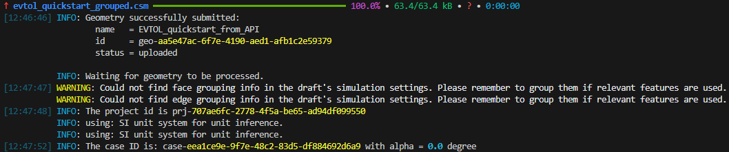
Output from running the API. Note that the IDs will be different when you run it.

The script will wait for simulation to complete. After completition, it will plot CL and CD convergence plot:

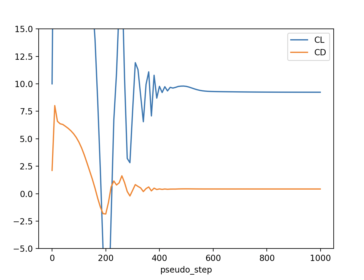
Force coefficient convergence plot.