Postprocessing a case with the WebUI#
Once a case has been run, we can now start doing the fun work: looking at the results.
Checking convergence#
The first thing to do is to check whether the case has converged succesfully. To do that we can look at the dashboard or the convergence tab. The convergence tab gives us the ability to monitor various metrics:
Nonlinear residuals: Turned on by default
Linear residuals: Shows convergence of the linear system of equation
CFL: Particularly useful when using Adaptive CFL
MinMax: Showcases the max residuals and their location for easy debugging
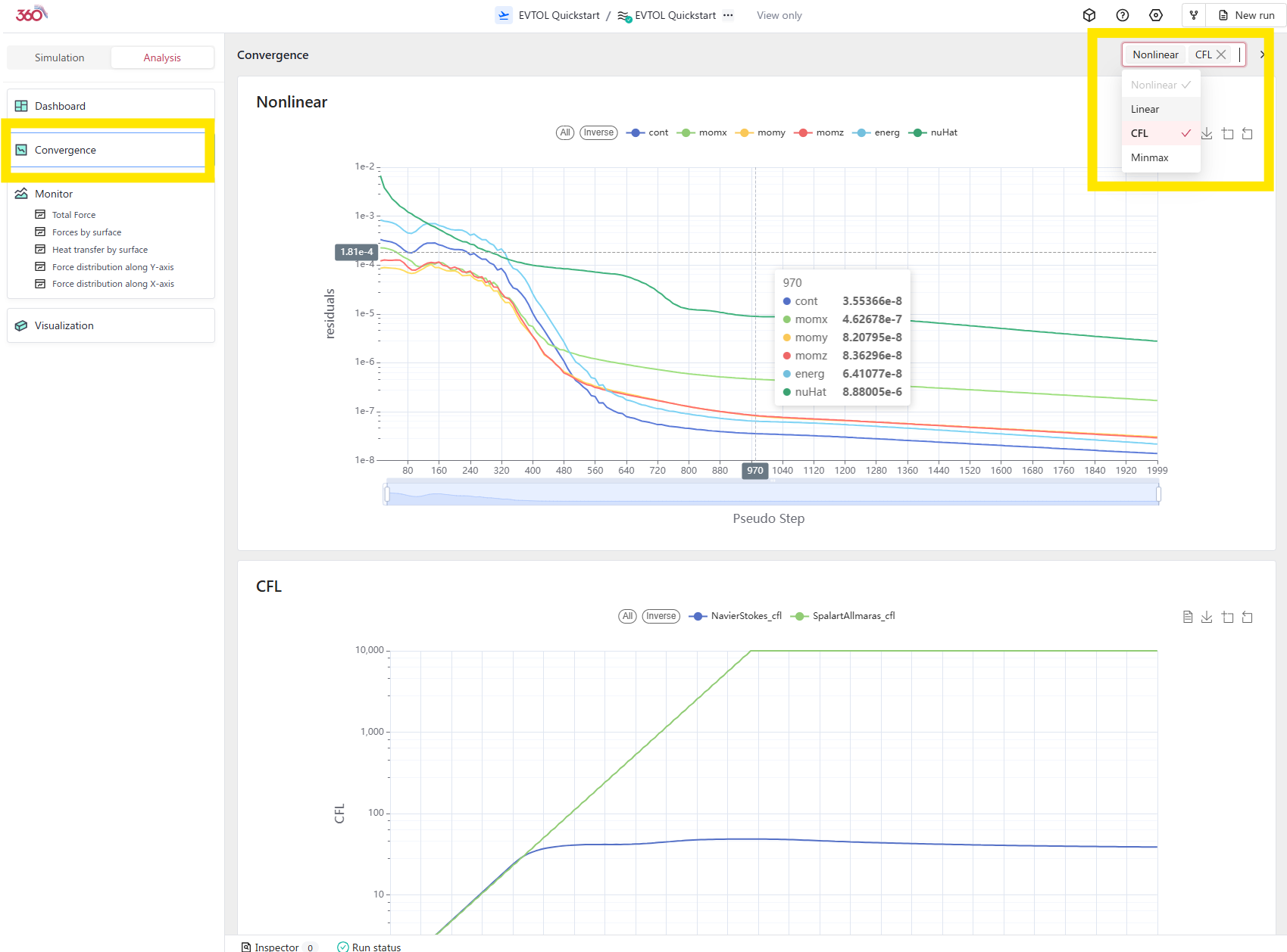
Checking a case’s convergence.#
Once we are comfortable that the case has converged, we can start to look at forces and visualize flow features.
Force History#
The Monitor module gives us the ability to look at various force history curves. In our case the interesting ones are:
Total Force: Shows the history of the summed forces on the vehicle
Forces by surface: If we had decomposed the airplane into sub components, we could analyse each component relative to each other.
Force distribution along Y axis: Shows the lift (or drag) vs span, which is useful to see how lift (or drag) is distributed.
Force distribution along X axis: Shows the drag (or lift) distribution vs length to see where drag (or lift) is being created.
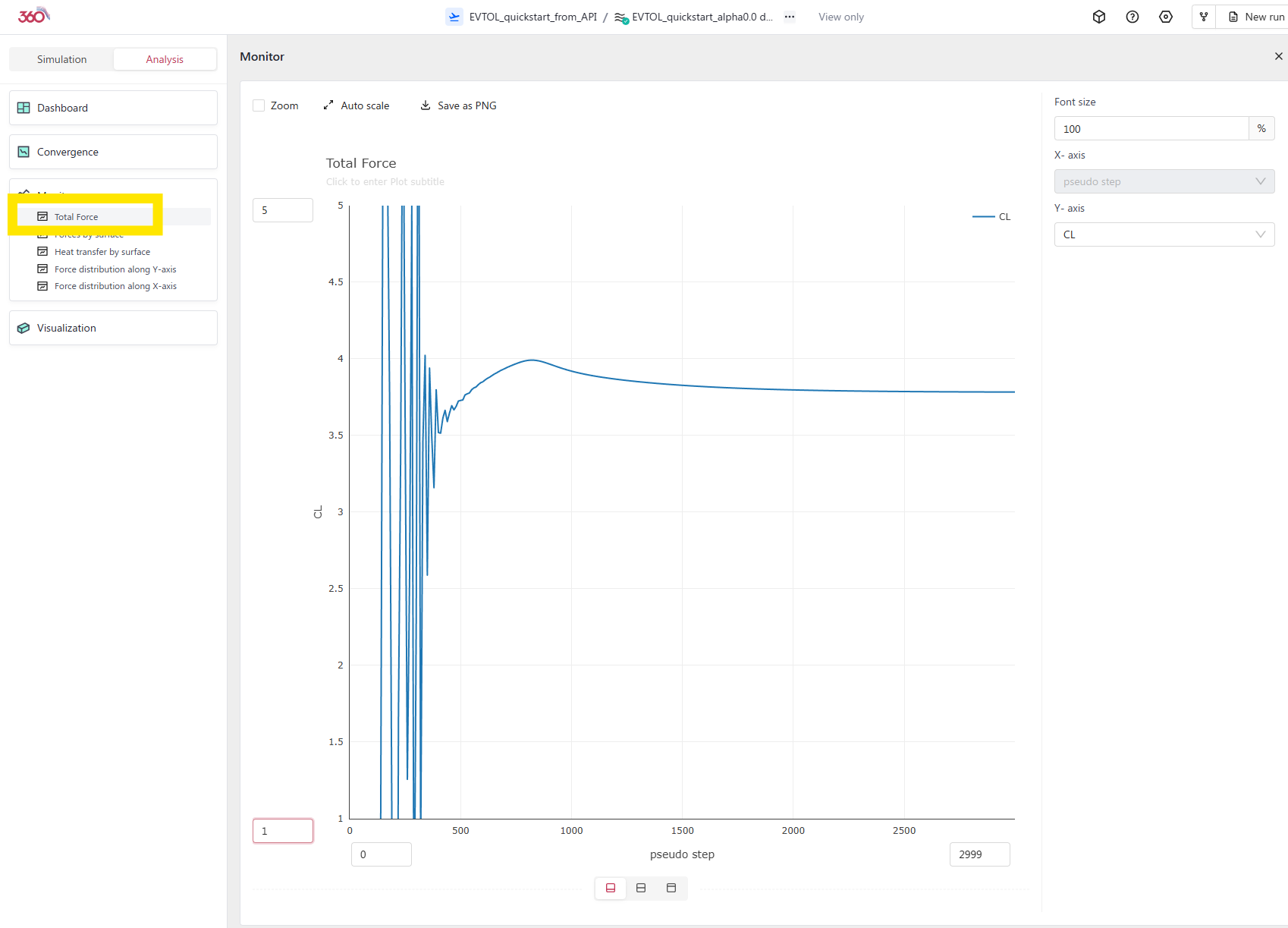
Total Lift history.#
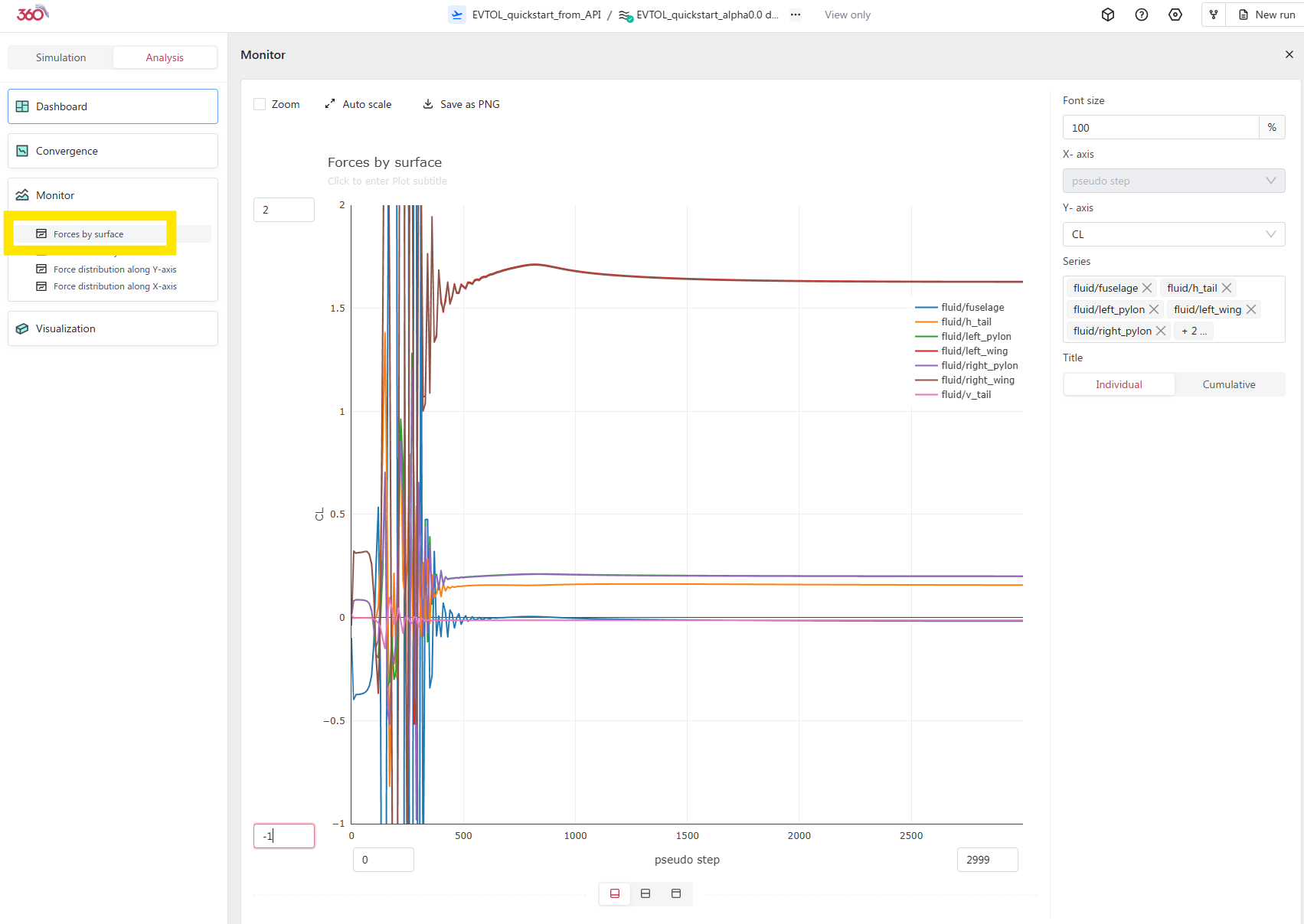
CL history for defined subcomponent surfaces.#
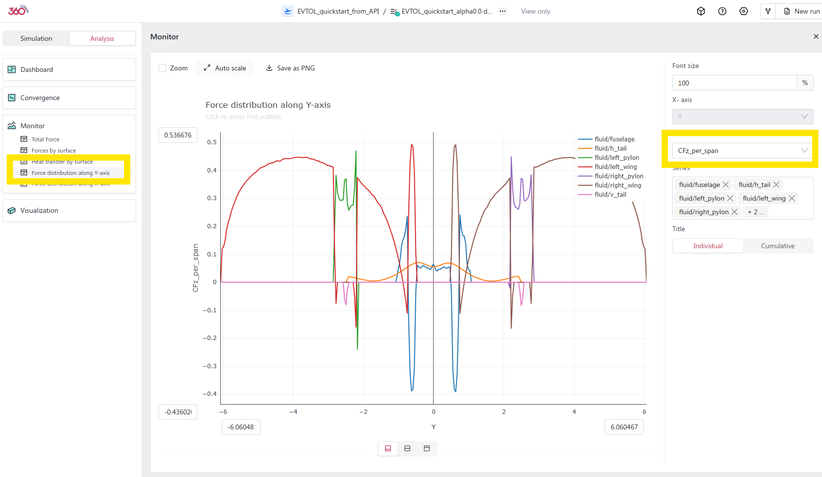
Lift vs span showing where the lift is being created. Notice the pylons’ negative effect on the lift distribution.#
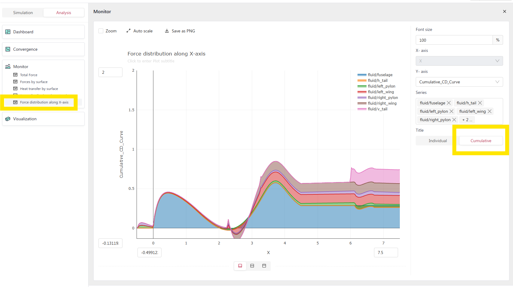
Drag vs length showing where the drag is being created.#
Visualization#
The visualization tab gives access to a powerful case visualizing set of tools.
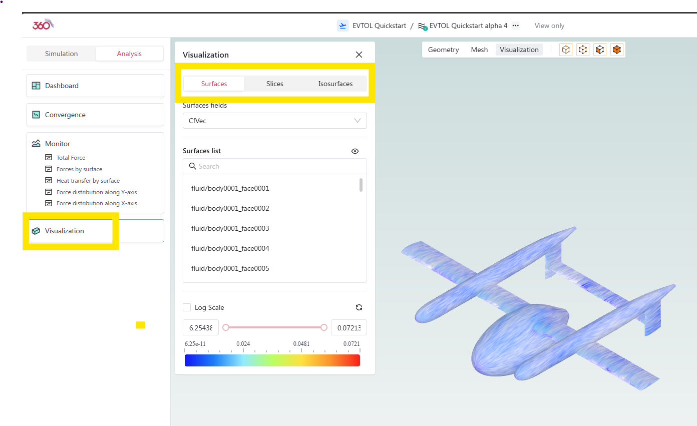
The visualization tab.#
the Visualization pop up gives us access to:
Surfaces:#
View the surface flow variables defined in surface outputs (see case output setup)
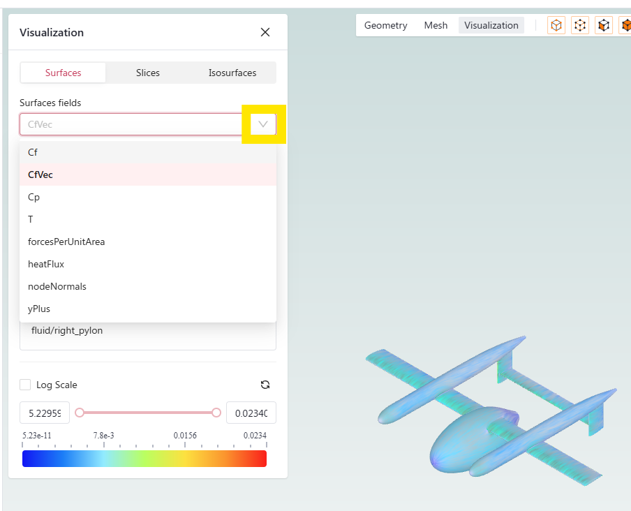
Viewing CfVec on the surface of eVTOL.#
Slices:#
If you have defined any output slices they will show up there. By default the solver generates three slices through the moment reference center. These slices can be turned on/off by clicking on the eye to open it or close it. The top eye affects all slices or they can each be turned on or off individually.
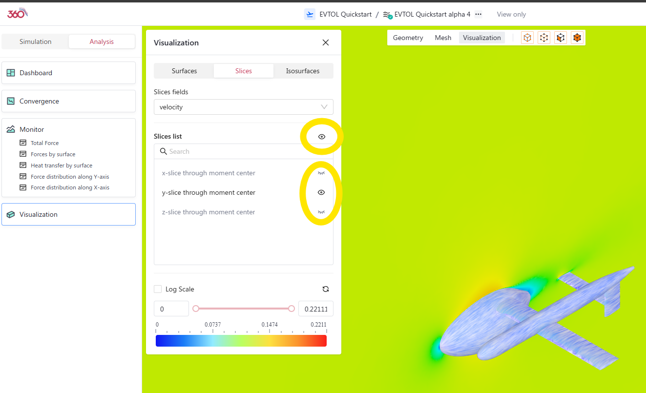
Viewing a constant Y slice.#
Isosurfaces:#
The solver automatically generates a Q_criterion isosurface to visualize where the vorticity is being shed. This is a very useful way of visualizing important flow features.
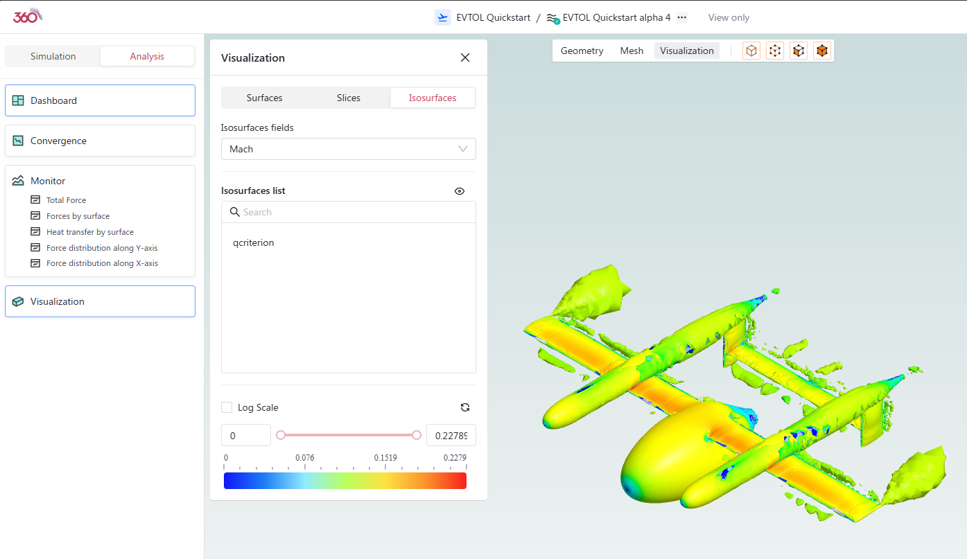
Viewing the Q-criterion isosurfaces.#
Comparing cases#
A very useful feature when comparing data across a variety of cases is the “case compare” feature. By going to our project tree, selecting the desired cases, and pressing the compare button, we can easily see the differences between the case setups and their results.
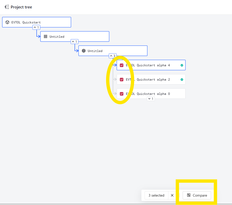
Comparing cases.#
By expanding and collapsing the input files we can easily compare what is different between each case. Notice how in our setup, only the alpha angle changes from one case to the next.
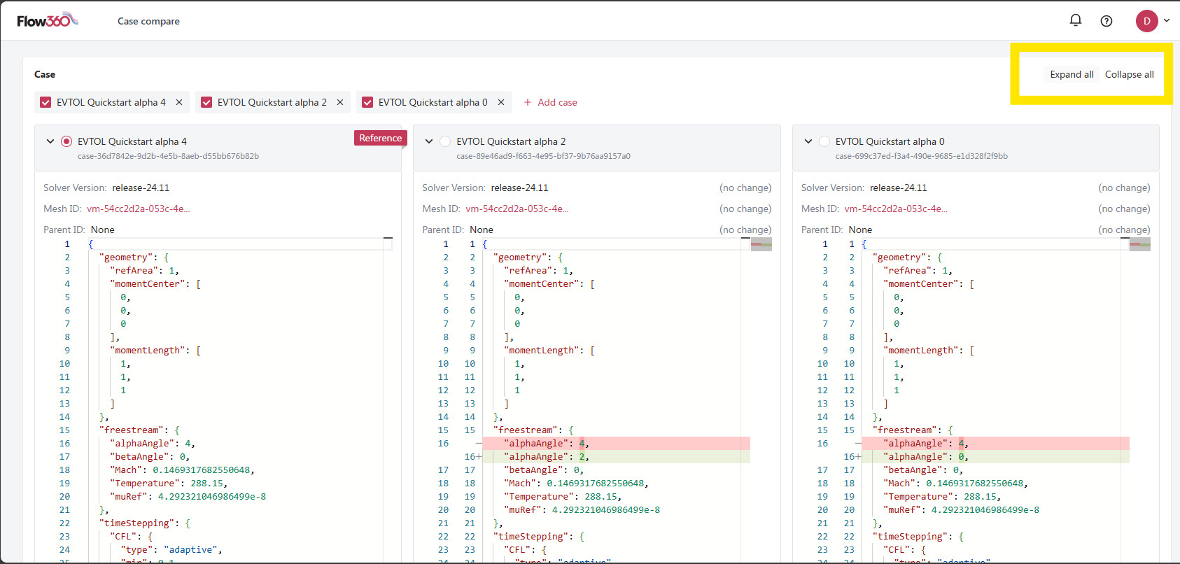
Comparing case inputs.#
If we collapse the inputs again we can see the automatically generated CL vs freestream.alphaAngle plot. That plot is highly customizable by changing the X-axis and Y-axis variables to plot.
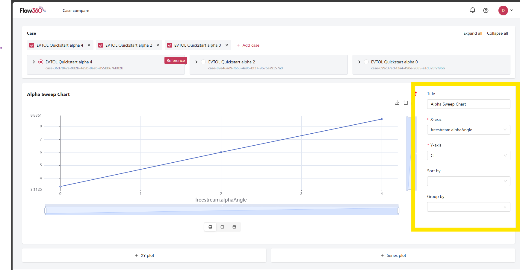
Plotting the results across multiple cases.#
One can generate additional XY plots by clicking on the + XY plot button. Another option is to generate a Series plot which shows the history of the selected variables for the various cases. In this example, we show the convergence history of all 6 residuals across the 3 cases, but we could also plot the force and moment histories or the values of the min/max values of the residuals.
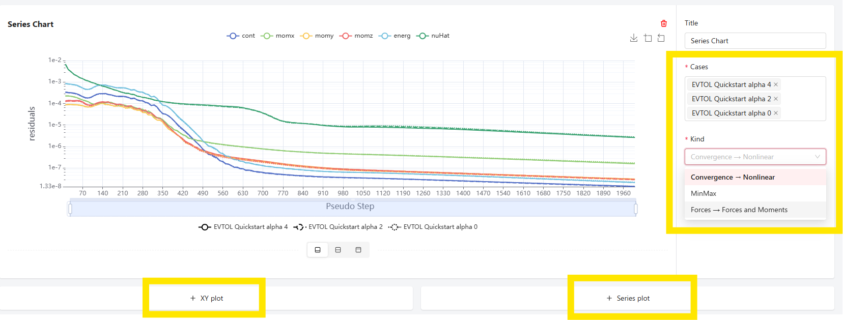
Plotting the convergence history.#
Project Assets#
All the files generated by the solver at the various steps of the import, meshing and running process are available to download. These include logs, results files, output csv tables etc…
To access those simply click on the cube in the top right of your screen. In the pop up window, scroll along the top to the particular entity you are interested in ( geometry, surface mesh, volume mesh or case) and then you will see all the files available for download. The most useful ones are usually the results/total_forces_v2.csv which contains the history of the aggregated forces on the vehicle and the results/surfaces_forces_v2.csv files that contains the force history on every single sub component comprising your vehicle.
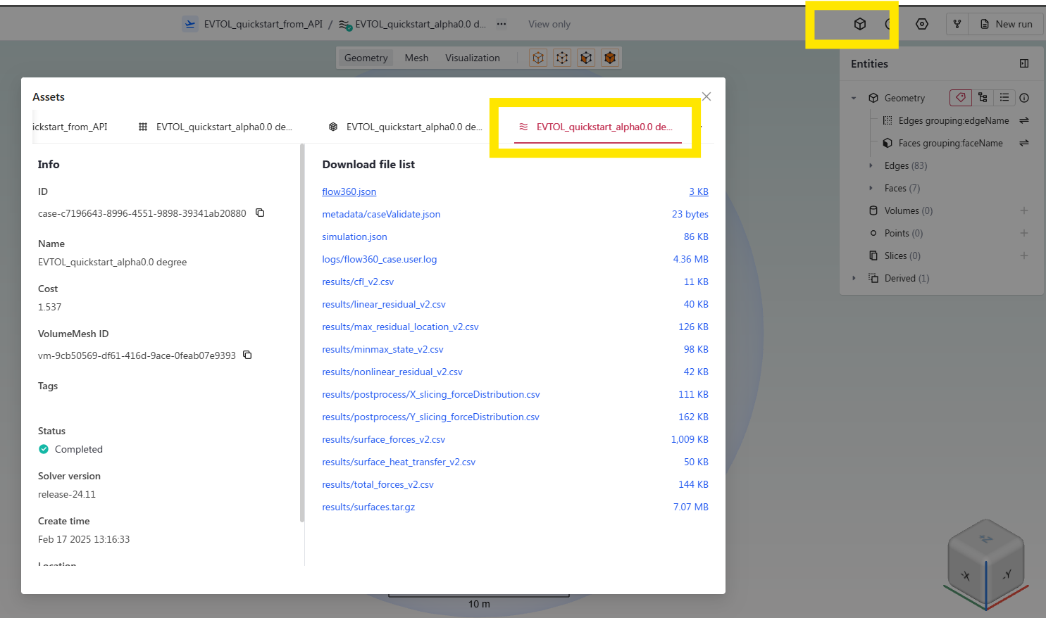
Accessing files to download.#
Congratulations on running your first Flow360 simulation 😄.