Launching a case with the WebUI

Now that we have generated a volume mesh, we can launch a case.

You will notice on the left hand side of the screen a panel containing 7 sections:

• Meshing: This topic was covered in the previous Quick Start tutorial

• Reference Geometry: Defines the reference lengths and areas.

• Operating Condition: Allows for the definition of the vehicle’s operating conditions.

• Models: Define the physics model to be used.

• Time Stepping: Covers steady state or time-accurate simulations along with all relevant time step criteria.

• User Defined Dynamics: Allow for custom expressions to calculate specific variables, as explained in this tutorial

• Output settings: Define the solution outputs that will be generated and available for download.

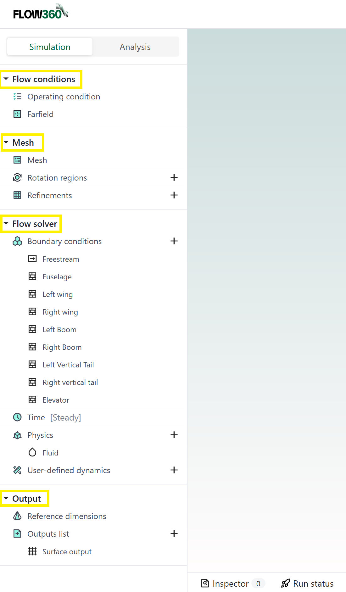
The 7 sections.

Creating a new run

We will now launch a new run by clicking the New Run icon and entering a run name in the ensuing popup and pressing submit.

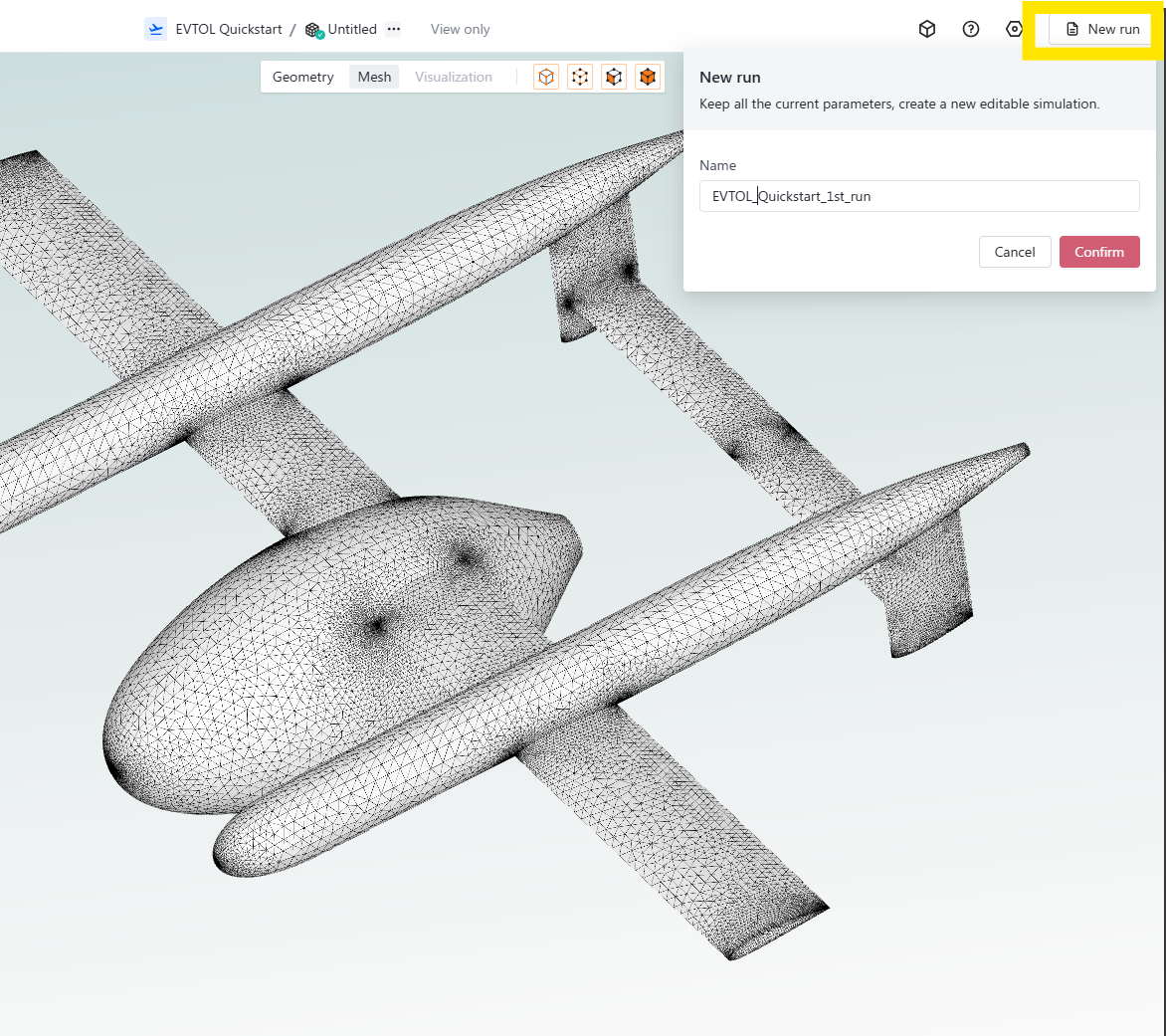
Creating a new run.

The Reference Geometry values are set by default to 1 meter for the reference lengths and 1 m ² for the reference area. Those values are adequate so we will leave them as they are.

For the Operating Condition, you will notice a little red dot pointing out that some values are missing. The inspector window in the bottom left also mentions that we have 1 error. In this case, we are missing a flow velocity value.

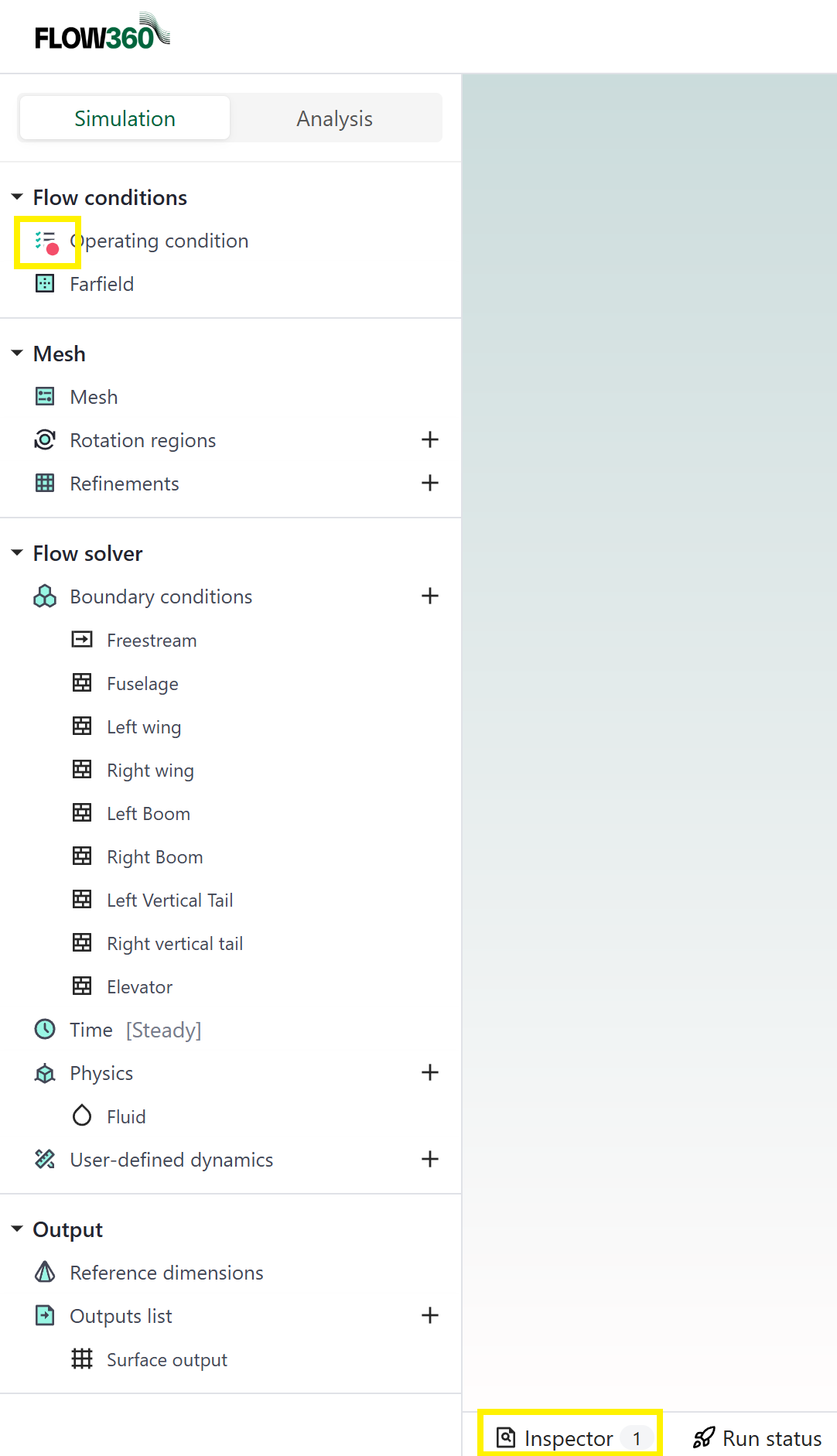
Notification that some required inputs are missing.

If we click on the inspector it opens up to reveal more information

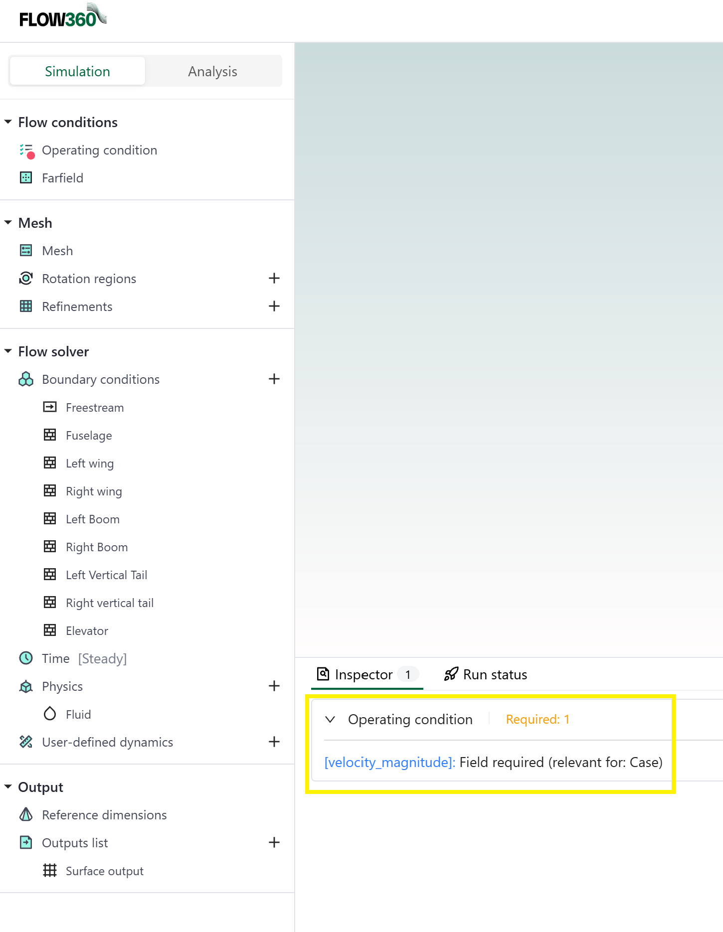
Inspector message outlining the missing inputs.

To rectify this, let’s click on the Operating Condition section and update the velocity to 50 m/s. The default \({\alpha}\) and \({\beta}\) flow angles along with more fluid properties can also be modified but we will leave them as they are.

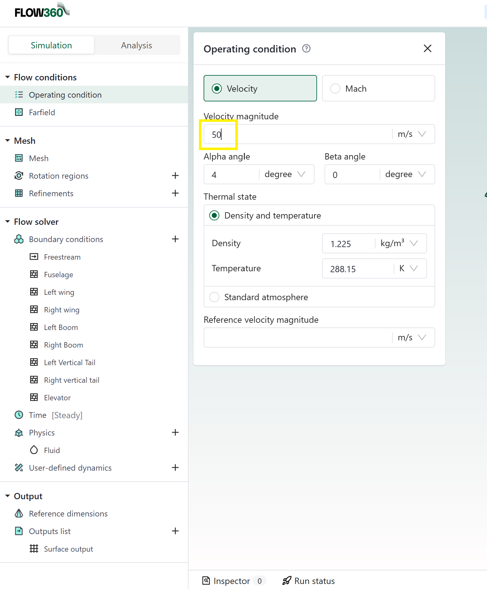
Entering the flow conditions.

We could change the type of simulation we do by adding components like virtual propellers models or others via the 3D models module.

The Time Stepping module allows us to select a steady state or time-accurate simulation and define how we do the time stepping.

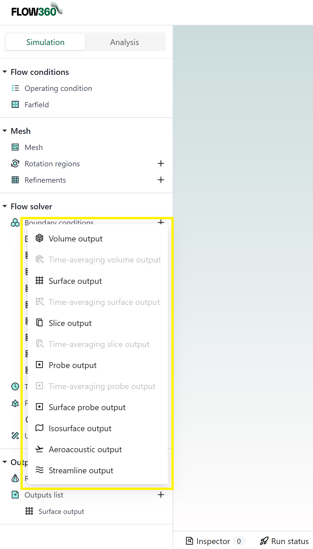
Last but not least, the Output Settings module lets you add a wide variety of output types depending on the type of data you require.

Entering the flow conditions.

Assigning boundary conditions

The web user interface gives us options to decompose the CAD entities into various sub components via the Boundary Conditions module.

Our eVTOL was decomposed in the following sub-components during the creation of .csm file:

• Fuselage

• Left wing

• Right wing

• Pylons

• Vertical tails

• Horizontal tail

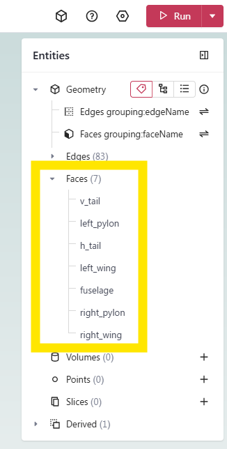
The 7 faces defining our EVTOL as defined in the CAD input .csm file.

As default we assign a no-slip wall boundary condition to all faces of the model to improve user experience. If needed the user can change the boundary conditions in this section.

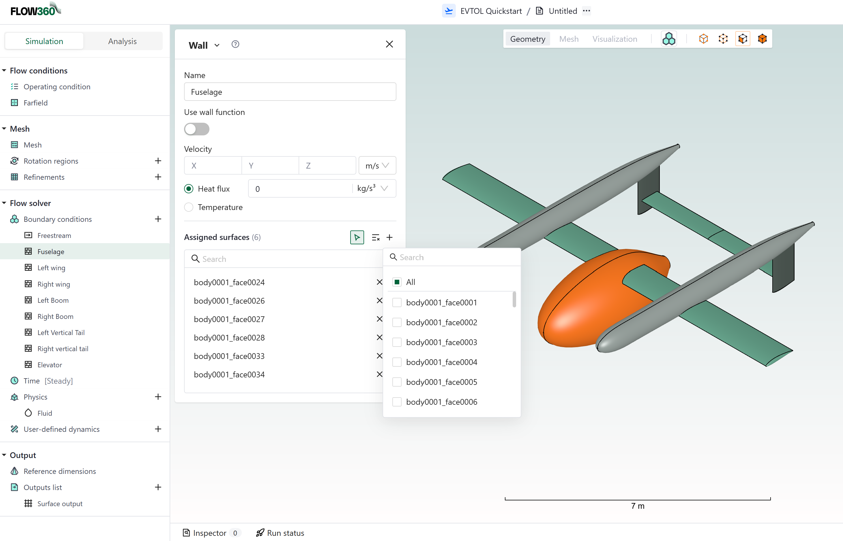
Default wall boundaries.

Now that we have defined the requirements, we are ready to click on the Run icon on the top right of our workspace and launch our simulation.

Tracking a case status

The case status can be tracked by looking at the Run status window at the bottom left of our screen next to the Inspector mentioned above.

You will notice that, as the run happens, your window will switch to the Dashboard view under the Analysis tab showing the most useful information all in one screen.

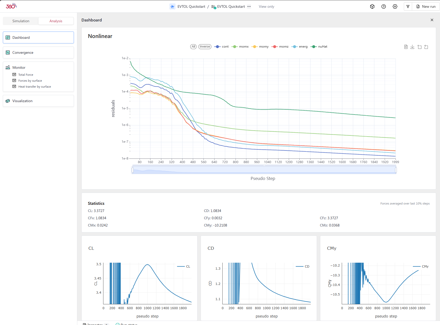
Run dashboard to monitor the most useful information.

forking a case

It may happen that you would like to continue a case for longer or restart a new case using a completed case as a startup. Both options can be done via the fork option. We will then be creating a child case that will have all the same settings as the parent case. We can then change some of settings if we so chose and Run the child case. If all we want to do is to continue the parent case for more iterations then we don’t need to change any settings, just fork and Run. To do so, simply press the fork icon, enter the child case’s name, confirm, change any of the settings on the left hand panes you so desire and press Run.

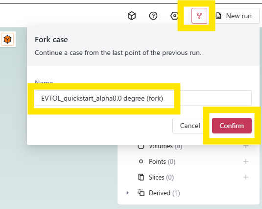
Forking an existing case

The project tree

A very useful feature for working within a project is the project tree that gives you quick access to all the entities in your project. The root is either the CAD geometry or volume mesh you uploaded. All the entities that have been generated off of that root are then displayed with their relative relationship clearly displayed. You can access the project tree by clicking on the project name in the top middle of the view.

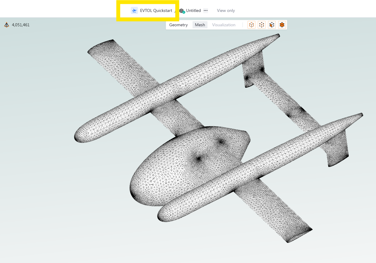
Accessing the project tree. Notice the volume mesh node count on the upper left of the window.

When the project tree opens you will find the root CAD geometry, the surface mesh and the volume mesh that derives from it. You can see here that if we created two more cases for alpha 2 and 4 the tree allows us to see all the cases we have run. You will notice also how the forked child case will be shown as dependent of its parent case. If you left mouse click on an entity you can bring up that entity in the workbench viewer and analyse it in more detail.

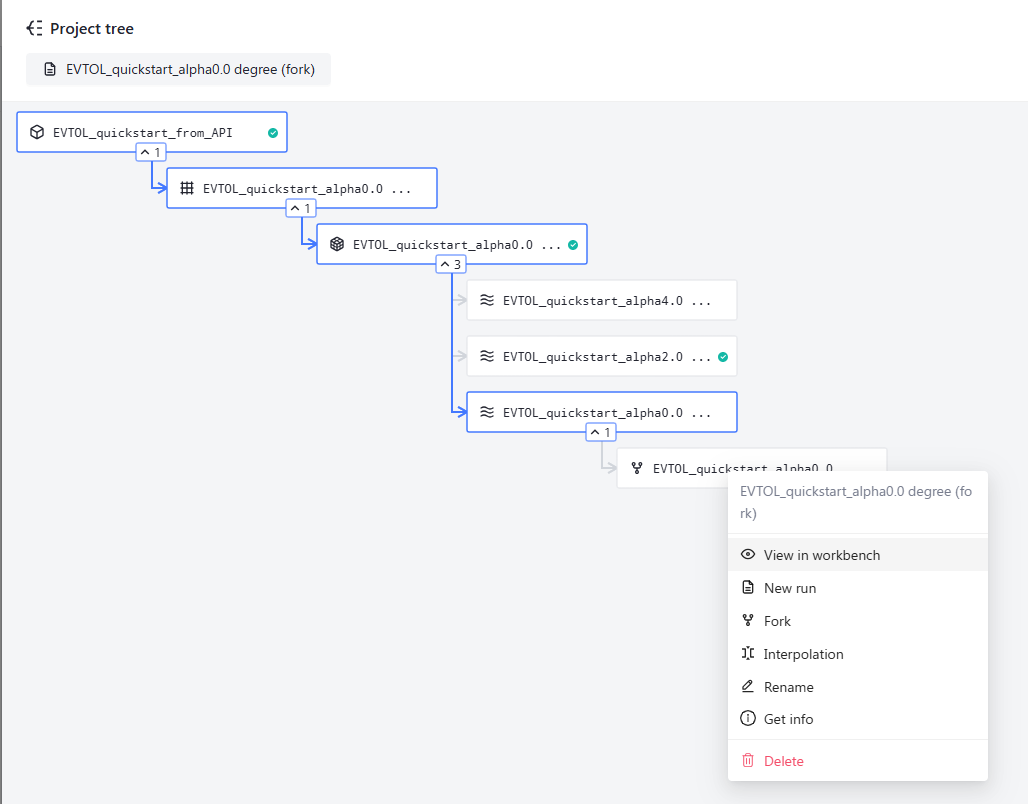
Using the project tree to navigate inside your project.

Now that we have run a case we will look at the result in the next Quick Start tutorial on post-processing