6.12. Aeroacoustics and Noise Simulation

6.12.1. Introduction

The main purpose of this case study is the verification and validation of the aeroacoustics and noise simulations with the Flow360 solver.

The flow around an aerodynamic body is governed by the Navier-Stokes equations, which express the conservation of mass, momentum, and energy. Direct Numerical Simulation (DNS) serves as a method for directly solving these equations. Achieving a comprehensive understanding of turbulent flow through DNS simulations demands a finely detailed grid and a small time step. The grid resolution must be fine enough to accurately capture the Kolmogorov length scale. In cases of isotropic turbulence, the grid requirements for a DNS simulation intensify in proportion to the Reynolds number. Furthermore, DNS simulations encounter challenges beyond computational intensity. The inherent complexity of turbulent flows, characterized by a broad range of spatial and temporal scales, necessitates the capture of intricate details. This requirement for high resolution in both space and time amplifies the computational burden. Additionally, DNS simulations require careful consideration of boundary conditions, which can be challenging to accurately model in realistic aerodynamic scenarios. These challenges collectively contribute to the current impracticality of employing DNS simulations in aeronautical applications.

In applications involving high Reynolds numbers, a widely adopted methodology involves categorizing turbulent flow characteristics into mean and fluctuating components, resulting in the derivation of the unsteady Reynolds-averaged Navier-Stokes (URANS) equations. This practical approach facilitates the computational representation of turbulent phenomena. The significance of turbulence modeling in this context is crucial. It contributes indispensably by providing necessary closure through the approximation of the Reynolds stress tensor within the URANS equations. Among the array of turbulence models, the Spalart-Allmaras (SA) model stands out for its widespread adoption in external aerodynamics, because it finds a good balance between being accurate and not taking up too much computer power. Consequently, the URANS framework, coupled with turbulence modeling, emerges as a valuable tool for the comprehensive simulation and comprehension of turbulent flows, particularly in practical engineering scenarios involving by high Reynolds numbers.

Studies have demonstrated that URANS lacks the capability to accurately predict unsteady flow behavior, particularly in cases of significant flow separation. Furthermore, its deficiency in scale-resolving capability limits its applicability for predicting broadband noise. Nonetheless, URANS can still be effectively utilized for design exploration and the prediction of tonal noise. Large-Eddy Simulation (LES) is commonly utilized for distinguishing larger turbulent motions from smaller scales. This is achieved by using a filter to partially resolve turbulence above a specific length scale. For scales below this threshold, turbulence is typically modeled empirically. When filtering is implemented, the filtered equations assume a similar form to the Unsteady Reynolds-Averaged Navier-Stokes (URANS) equations. The sub-grid stress tensor becomes crucial in LES, as it characterizes the unresolved scales and necessitates a modeling approach. Filtering can be explicitly applied by using a Sub-Grid-Scale (SGS) model to represent the unresolved sub-grid scale, or implicitly through the utilization of numerical dissipation in discretization as a low-pass filter. In simpler terms, implicit filtering acts as a filter with a local grid spacing. When considering implicit Large-Eddy Simulation (LES), no explicit SGS model is incorporated. LES is a commonly employed method for aeroacoustic simulation, as it effectively resolves a broad range of large turbulent eddies. However, it’s important to note that the grid resolution requirements for LES simulations of high Reynolds number flows scale proportionally with the Reynolds number and are considered computationally expensive. More information about the influence of Reynolds number on drag coefficient can be found in drag crisis.

In this case study, the URANS, ILES, and DDES approaches are applied to different applications, and the outcomes are compared against experimental results. The following sections are presented in this documentation:

1. First Part: Cylinder Case:

   • Comparison of pressure fluctuations

   • CFD-FWH vs. Direct-CFD

   • Verification using URANS approach

2. Second Part: Rod-Airfoil Configuration:

   • Validation of acoustic solver against experimental data

   • Utilizing ILES approach

3. Third Part: Two-Bladed Propeller Test Case:

   • Further validation of acoustic solver against experimental data

   • Incorporating ILES and DDES approaches

6.12.2. Cross Flow over Circular Cylinder

In this instance, we validate the accuracy of the flow and acoustic solver (CFD-FWH). The freestream Mach number is set at 0.25, accompanied by a Reynolds number of \(5 \times 10^{6}\).

Fig. 6.12.1 illustrates the boundary conditions, mesh resolution, and microphone locations.

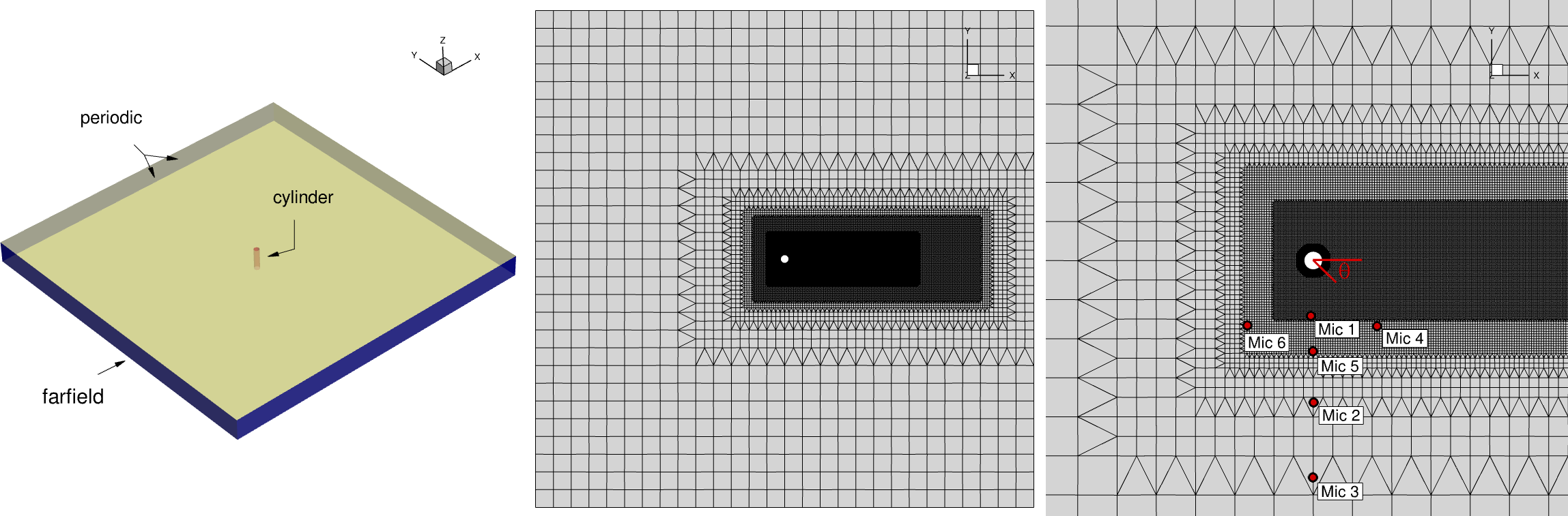
Fig. 6.12.1 Summary of boundary conditions, mesh details, and microphone locations for the cross-flow over the circular cylinder case.

We used periodic boundary conditions with a spanwise length of \(L_{z}\) = 4 \(\times\) D. The mesh node statistics are detailed in Table 6.12.1.

Table 6.12.1 Grid properties for cross flow over the cylinder.

Grid	Circumferential	Spanwise	Boundary Layer	Total
A	500	100	500×46	7.5M

The purpose of this test case is to validate the acoustics results by comparing pressure fluctuations obtained from the acoustic solver with those directly extracted from the CFD data. In simulating the unsteady flow, URANS with the SA turbulence models is employed, using a second-order dual time-stepping method with a time step size of \(\frac{0.2 D}{c_{\infty}}\), corresponding to 100 time steps per vortex-shedding cycle.

Flow360’s acoustic solver computes pressure fluctuations at six microphone locations. Specifically, three microphones are radially positioned at a constant polar angle, while three are placed circumferentially at an equal distance from the cylinder. In Fig. 6.12.1, microphone locations are highlighted with red dots. Detailed positions can be found in Table 6.12.2. The objective is to verify and validate the results of the acoustic solver against direct CFD data extraction.

The FWH equation is applied using only the “dipole” source terms on the cylinder surface (the Curle approximation at low Mach numbers). The FWH equation was derived for 3D bodies finite in all directions, which this body is not. To reflect this, the pressure fluctuations in the acoustic region are calculated by adding the integral calculated on the primary cylinder of length 4D and the integrals calculated on a number of periodic “images” in both directions spanwise. As the image goes to large distances, its contribution dwindles and the series converges. This is crucial to the comparison with the (periodic) simulation field itself. In particular, for a finite body the pressure signal (\(p^{\prime}\)) decays like 1/r for large r, but for 2D and periodic situations it decays only as fast as 1/sqrt(r). This was verified for microphones 1, 5, 2, and 3.

Table 6.12.2 Microphone positions around the cylinder.

Microphones	r	θ
1	3D	90°
2	6D	90°
3	12D	90°
4	5D	45°
5	5D	90°
6	5D	135°

The comparison of pressure fluctuations at the three microphones at the same radial distance from the cylinder is illustrated in Fig. 6.12.2.

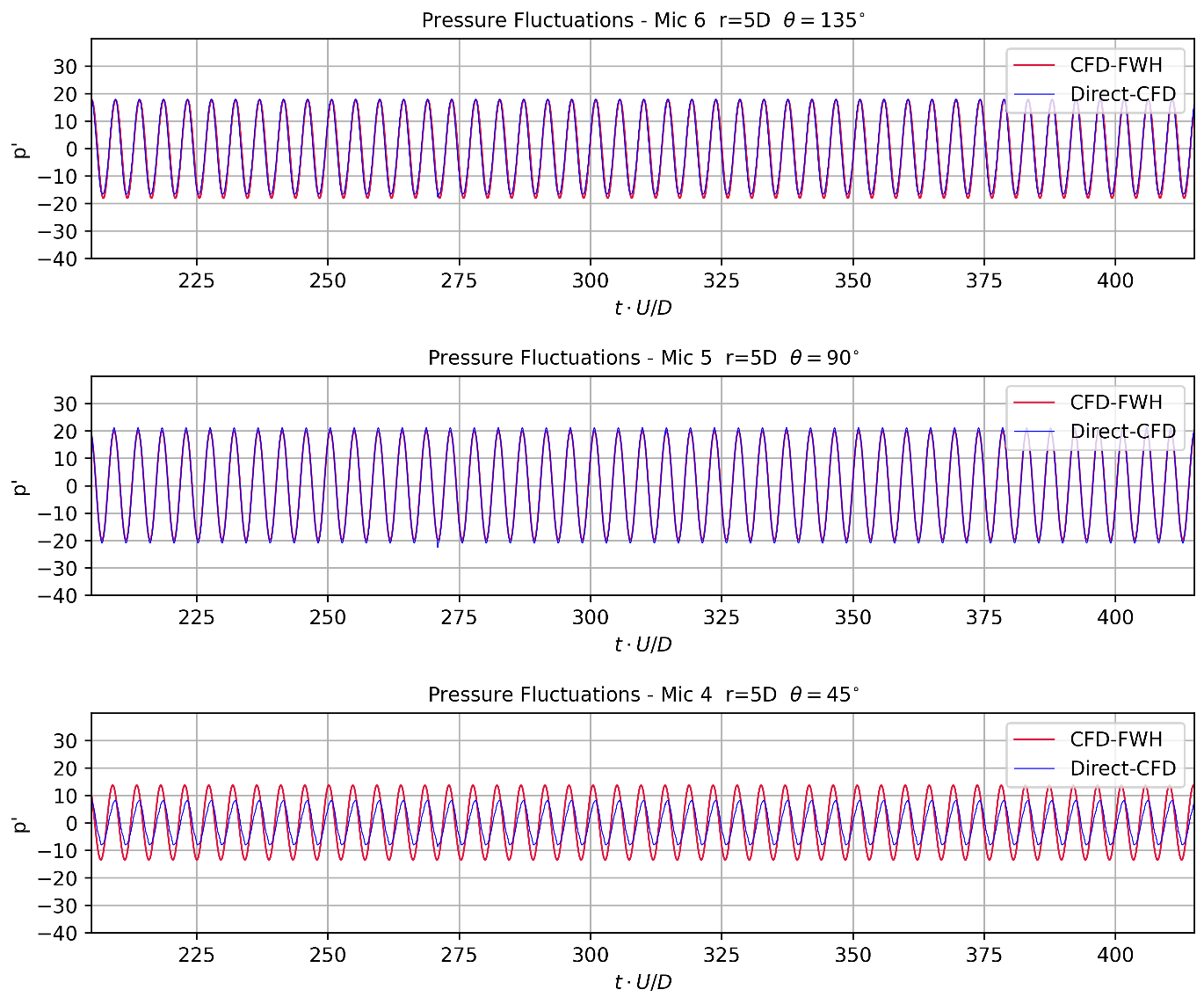
Fig. 6.12.2 Pressure fluctuations for microphones at the same radius for the cross flow over the circular cylinder.

The frequency matching for pressure fluctuations from both the CFD solver and acoustic solver is excellent for all three radial observers. However, a discrepancy in amplitude is observed at microphone 4, tentatively attributed to the increased impact of 3D turbulent flow downstream of the body, where this observer is positioned. The Quadrupole source terms which were ignored are strong in that region.

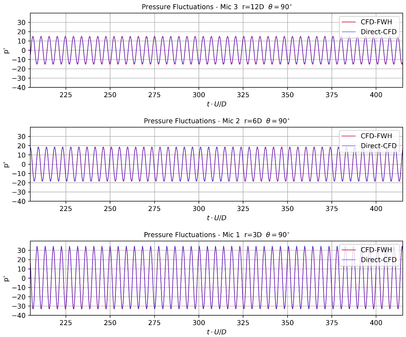
Fig. 6.12.3 Pressure fluctuations for microphones at the same angle for the cross flow over the circular cylinder

Meanwhile, the pressure fluctuations at three microphones at the same angle are illustrated in Fig. 6.12.3. Frequency alignment is observed for all three radial microphones, with a slight mismatch in amplitude at microphone 3 due to mesh coarsening. Furthermore, a \(p^{\prime}\) scaling proportional to \(1/\sqrt{r}\) is achieved. The internal consistency test is successful.

This comparison underscores the equivalence of pressure fluctuations from the acoustic solver to those directly computed from CFD calculations. However, emphasizing the importance of mesh resolution in the near-field region, the accuracy of CFD-FWH results is contingent upon the quality of the unsteady CFD calculation.

6.12.3. Rod-Airfoil Configuration

The rod-airfoil configuration serves as a standard benchmark for investigating the interaction noise between different aircraft components. Jacob et al. ¹ conducted the experiment in the wind tunnel at Ecole Centrale de Lyon (ECL). The primary goal of these experimental tests was to establish a comprehensive database against which CFD/CAA methods could be benchmarked. In the study conducted by Jacob et al., they simulated basic geometric elements, resulting in two distinct types of noise: quasi-tonal noise due to the periodic shedding of vortices at the rod and broadband noise caused by the turbulent wake impinging on the airfoil. This setup provides a means to assess the CFD code’s accuracy in predicting the shedding frequency of vortices from a bluff body and modeling the decay of turbulent structures in the wake. Widely employed for validating numerical methods in airframe noise prediction, this configuration is a prevalent reference in the field.

As per Jacob et al., the rod generates a von Kármán vortex street with a Strouhal number (\(St\)) of \(St=0.19\). The rod’s boundary layer maintains laminar characteristics, transitioning to turbulence in the wake. Instability waves emerge in the shear layers, engaging with two-dimensional structures. The ensuing turbulent wake interacts with the airfoil’s leading edge, positioned one chord downstream.

Impinging on the airfoil, the large vortices split and form two smaller eddies, passing above and below the airfoil. Smaller vortices undergo distortion and don’t make direct contact. Consequently, both direct and non-direct interactions between vortices and the airfoil can be examined. These interactions induce unsteady loads on the airfoil and alter the acoustic spectrum. Comparing the rod-airfoil configuration to the rod-only setup, the sound pressure level’s tonal peak is higher in the former. The smaller vortices, significantly smaller than the airfoil’s maximum thickness, introduce a broadband component to the spectrum. Furthermore, the tonal peak broadens due to the development of turbulence and the nonlinear effects of large vortices on the airfoil’s leading edge.

Various researchers have undertaken comparisons among URANS, LES, and DES methodologies for this specific test case. Casalino et al. ² investigated unsteady compressible RANS simulations, while Peth et al. ³ utilized a compressible implicit LES solver for their numerical study. Galdeano et al. ⁴ conducted a study employing a compressible DES based on the SA turbulence model. According to Giret et al. ⁵, given that the boundary layer’s transition to turbulence and its detachment significantly impact shedding frequency, unsteady loads, and consequently the acoustic pressure spectrum, the effectiveness of the DES method may hinge on the model used to resolve boundary layers around the bluff-body. They investigated the specified configuration employing an unstructured compressible Large Eddy Simulation (LES) code. Their study involved a comparative analysis of the influence of spanwise dimension and the sensitivity of rod/airfoil alignment on the prediction of noise.

In our case study, we chose compressible implicit LES simulations to predict the acoustic pressure spectrum. The simulations are carried out using the Flow360 code, which is an unstructured compressible solver. Both Roe and low-dissipation Roe are used in this case study. Our study’s primary aim is to evaluate the effectiveness of Flow360, coupled with the Ffowcs-Williams and Hawkings (FWH) code, in calculating far-field noise. Given our focus on evaluating far-field noise, using direct-CFD approach, similar to the cylinder test case in the previous section, becomes unfeasible. This is attributed to the necessity for a refined mesh across a considerable domain capable of propagating acoustic waves. We intend to compare our findings with experimental data and other numerical results available in the existing literature.

6.12.3.1. Simulation Setup

In this specific test case, the rod-airfoil configuration consists of a NACA0012 airfoil with a chord (C) of \(C=1 m\) and a cylindrical rod with a diameter (d) of \(d=0.1C\) that positioned one chord upstream. The flow conditions encompass a uniform airflow with \(U_{in}=72 m/s\), \(T_{in}=293 K\), and \(\rho_{in}=1.2 kg/m^{3}\). The Reynolds numbers based on the rod diameter (\(Re_{d}\)) and the airfoil chord (\(Re_{C}\)) are \(Re_{d}=4.8\times10^{4}\) and \(Re_{C}=4.8\times10^{5}\) respectively. The spanwise length is \(5d\).

Fig. 6.12.4 illustrates the boundary conditions, mesh resolution, and microphone locations.

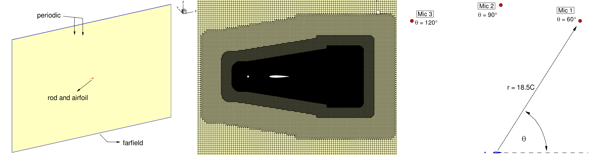
Fig. 6.12.4 Summary of boundary conditions, mesh and microphone locations for the rod and airfoil test case.

We implemented periodic boundary conditions with a spanwise length (\(L_{z}\)) of \(L_{z}\) = 5 \(\times\) d. Detailed mesh node statistics can be found in Table 6.12.3. Although a mesh refinement study around the rod was conducted, it is not presented in this particular case study.

Table 6.12.3 Grid points for the rod and airfoil test case.

Grid	Rod	Airfoil	Spanwise	Rod BL	Airfoil BL	Total
A	1000	1018	200	1000×49	1018×49	88.1M

6.12.3.2. Aerodynamic Validation

The iso-surface of Q-criterion plot shown in Fig. 6.12.6 reveals the vortex-shedding structure impinging on the airfoil. Displayed in Fig. 6.12.5 is the time-averaged pressure coefficient over the rod. A comparison is made between Implicit Large Eddy Simulation (ILES) with and without a low-dissipation scheme, and the experimental results provided by Travin et. al ⁶. In both simulations, a notable accord is observed when evaluating against the experimental data. Particularly noteworthy is the ILES with a low-dissipation scheme, which demonstrates a marginally superior agreement beyond \(\theta\) = 60 °.

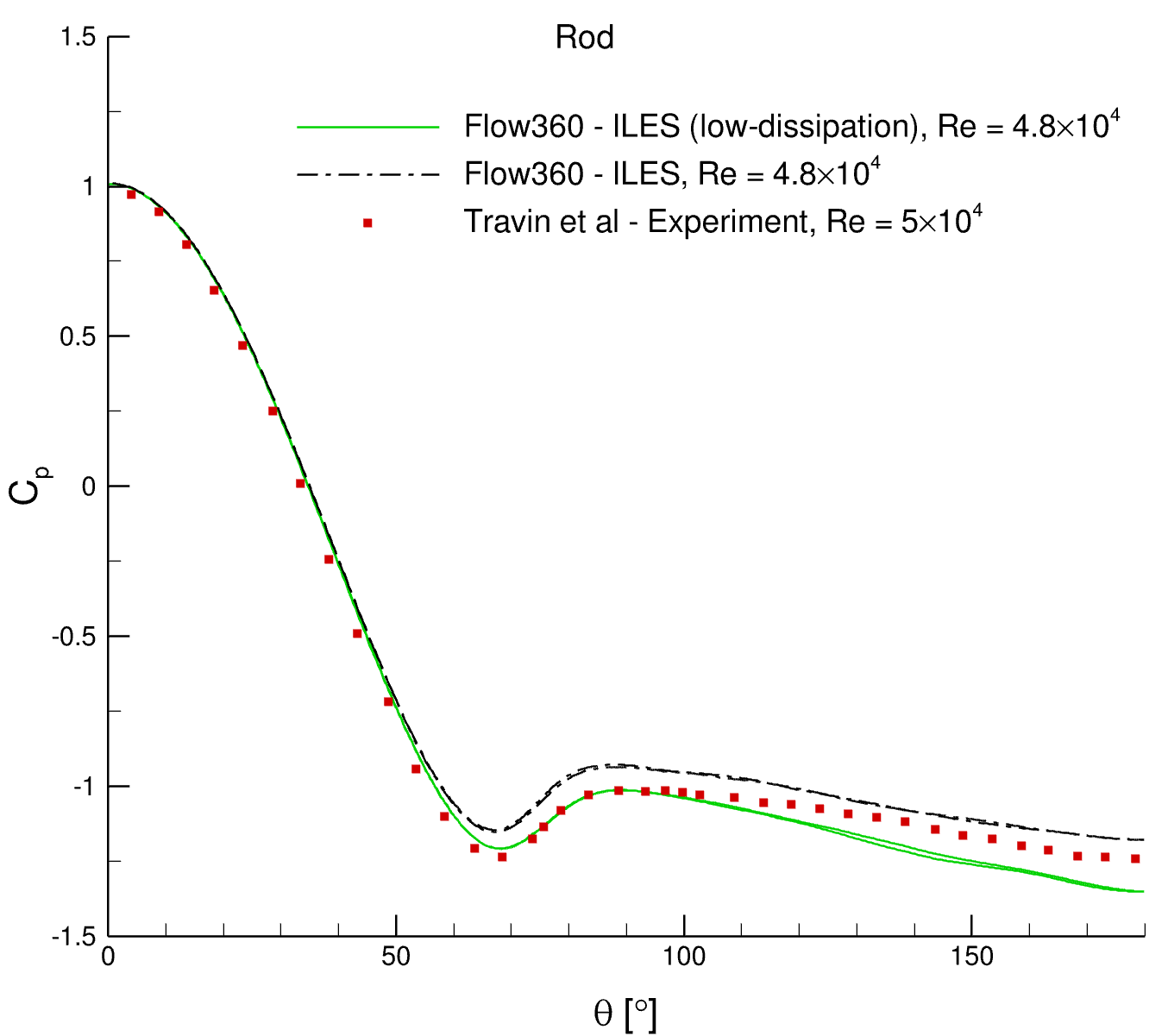
Fig. 6.12.5 Time-averaged pressure coefficient \(C_{p}\) obtained from ILES simulations with Roe and LDRoe schemes around the rod at Re= \(4.8 \times 10^{4}\).

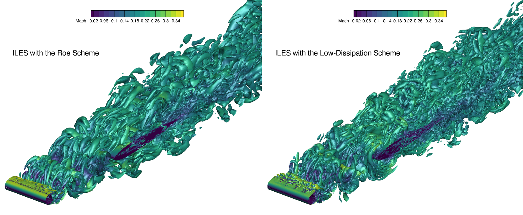
Fig. 6.12.6 Iso-surfaces obtained from ILES simulations with and without the low-dissipation scheme at Re= \(4.8 \times 10^{4}\).

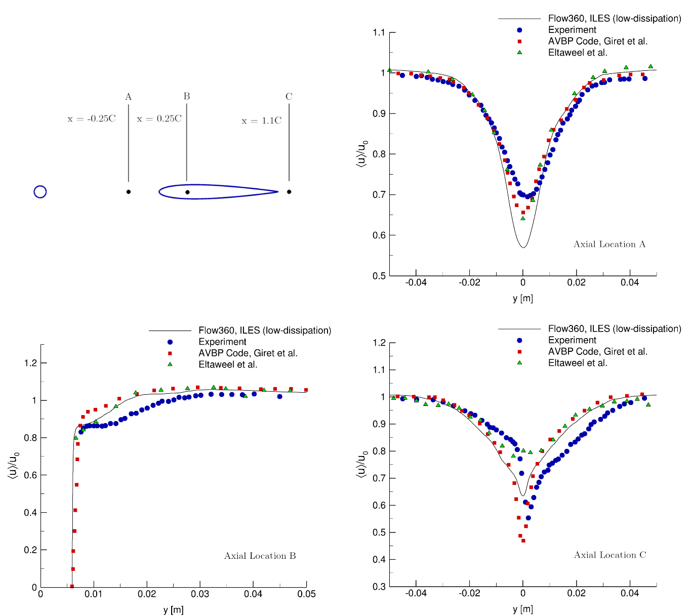
Fig. 6.12.7 Velocity profiles comparison against experiment at three axial locations obtained from ILES simulation with LDRoe scheme for the rod and airfoil test case.

An assessment is conducted at three axial locations, as depicted in Fig. 6.12.7, to facilitate a comparative analysis of velocity profiles against experimental data. The corresponding velocity profile comparisons are presented within the same figure. A fair agreement in mean velocities is discerned when evaluating against the experimental data.

6.12.3.3. Noise Evaluation

The acoustic power spectral density (PSD) for angular positions 60 °, 90 °, and 120 ° is presented in Fig. 6.12.8. The numerical results exhibit a commendable match with both experimental data and other numerical results available in the literature across all microphone angular positions. Similar to the cylinder case in the first section, the pressure fluctuations in the acoustic region are calculated by considering a number of periodic “images” in both directions spanwise.

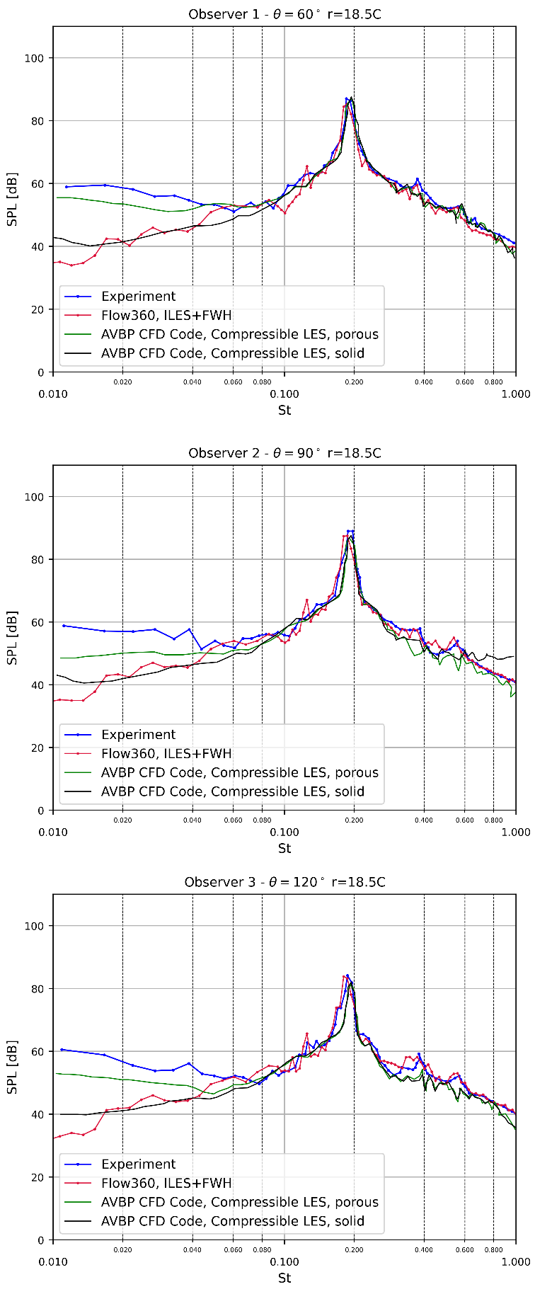
Fig. 6.12.8 Acoustic PSD comparison against experiment at different microphone positions obtained from ILES simulation with LDRoe scheme for the rod and airfoil test case.

The Strouhal peak is effectively captured for the two source surfaces. The computed Strouhal number based on the Sound Pressure Level (SPL) spectra for three observers is \(St=0.186\), which is in good agreement with the experimental value of \(St=0.19\). However, a more noticeable discrepancy at higher frequencies is observed, particularly at the downstream microphone (\(\theta\) =60 °). This test case underscores the reliability of acoustic simulation using Flow360 with an Ffowcs-Williams and Hawkings (FWH) acoustic analogy for predicting noise in a rod-airfoil configuration. The compressible Implicit Large Eddy Simulation (ILES) with a low-dissipation scheme on an unstructured mesh allows for high-fidelity resolution of acoustic sources and their propagation. The FWH analogy efficiently extrapolates the pressure field in the far-field region at a relatively small computational cost. Meanwhile, the CFD-FWH method proves effective in predicting both the tonal and broadband components of the sound generated by the rod-airfoil configuration.

6.12.4. Two-bladed Propeller

With the rise of Urban Air Mobility (UAM), accurately predicting noise from propeller systems is crucial. CFD simulations for UAM propellers differ significantly from more conventional aircraft, involving lower tip speeds and intricate three-dimensional flow features like transitions, separations, and crossflows. The lower tip speeds make the prediction of broadband noise from trailing edge separation particularly important. The complex three-dimensional flow features underscore the need for using high-fidelity CFD methods for noise prediction, raising doubts about the reliability of lower-fidelity methods like Blade Element Momentum Theory (BEMT) and Nonlinear Vortex Lattice Method (NVLM). Precisely predicting broadband noise relies on effectively capturing turbulent fluctuations both in the boundary layer and the wake, highlighting the importance of scale-resolving approaches.

In this case study, we explore the far-field noise signature of a two-bladed open propeller manufactured by Mejzlik, using Flow360 and its acoustic solver based on the Ffowcs-Williams and Hawkings (FWH) analogy. The propeller, with a diameter (\(D_{p}\)) and pitch (\(P\)) of 9 inches (\(9\times9\)) , was experimentally studied at the University of Bristol Aeroacoustic Facility, with results reported by Baskaran et al. ⁷.

6.12.4.1. Simulation Setup

This study considers two operating conditions, representing hover and forward modes, with freestream velocities of \(0\) and \(15 m/s\). The CFD domain and the specified boundary conditions are illustrated in Fig. 6.12.9.

The Reynolds numbers based on the chord length at \(75\%\) of span (\(Re_{75}\)) and based on the propeller’s diameter (\(Re_{D}\)) and tip Mach number (\(M_{tip}\)) of 0.21 is \(Re_{75}=62816\) and \(Re_{D}=1121855\) at hover mode. At forward mode they are: \(Re_{75}=64172\) and \(Re_{D}=1146072\).

The advance ratios at hover and forward modes are \(\frac{U_{\infty}}{nD_{p}}=0.00\) and \(0.66\), with the propeller rotating at \(6000 rpm\) for both conditions. The \(U_{\infty}\) is the freestream velocity in \(m/s\), \(n\) is the rotational speed of the propeller in revolutions per second, and \(D_{p}\) is the propeller’s diameter in \(m\). The blade-passing frequency (BPF) is 200Hz, and the blade tip Mach number is \(0.21\). Additional freestream properties include \(p_{\infty} = 101325 Pa\), \(T_{\infty} = 288.15 K\), and \(\rho_{\infty} = 1.2 kg/m^{3}\).

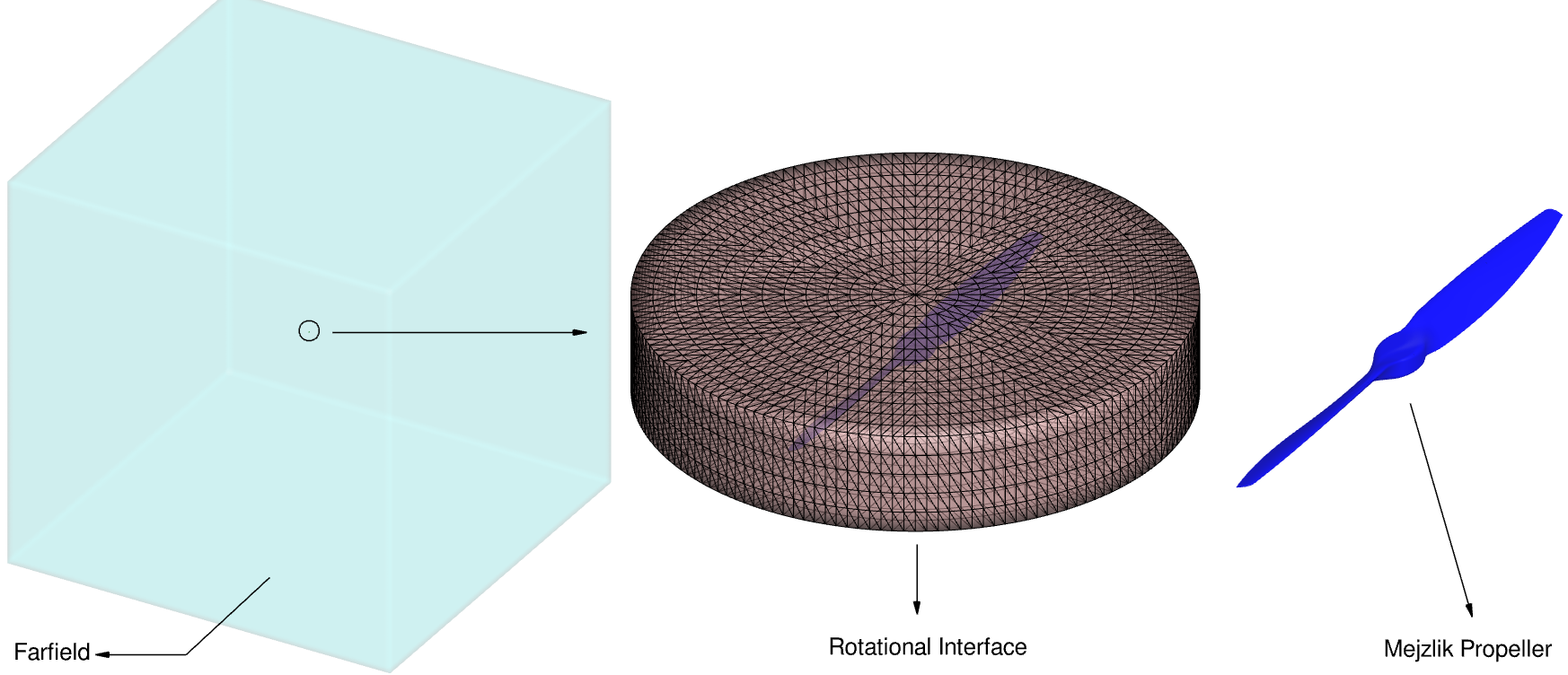
Fig. 6.12.9 Summary of boundary conditions for the two-bladed Mejzlik propeller.

6.12.4.2. Grid Refinement Study

In the overall process, four unstructured grid levels are generated using a hex-dominant algorithm both in the near-field and the far-field. The surface mesh utilized for this case study is a quad-dominant unstructured mesh designed to accurately capture the rounded leading-edge and the trailing-edge of the propeller geometry through anisotropic stretching. This stretching is specifically applied to the surface based on the edge boundaries of the propeller geometry.

Four refinement zones are strategically placed around the propeller to maintain control over mesh coarsening, facilitating a gradual increase in cell edge length in the wake region. This measured coarsening of the mesh in the wake region aids in dissipating vortical structures and preventing residual acoustic reflections that may not be sufficiently damped by non-reflective boundary conditions. Across different grid levels, the mesh undergoes refinement in all directions, covering both the surface mesh and refinement zones. The mesh node statistics for three mesh levels are detailed in Table 6.12.4, with mesh level 1 visually represented in Fig. 6.12.10.

Table 6.12.4 Grid point statistics for the mesh refinement study.

Grid	GR	Initial Height	Mesh y+	Surface Points	Total Points
Level 0 (coarse)	1.1	0.000001	1	331K	19.2M
Level 1 (medium)	1.09	0.0000005	1	947K	59.6M
Level 2 (fine)	1.07	0.0000005	1	1340K	111M
Level 3 (extra fine)	1.07	0.0000005	1	1901K	188M

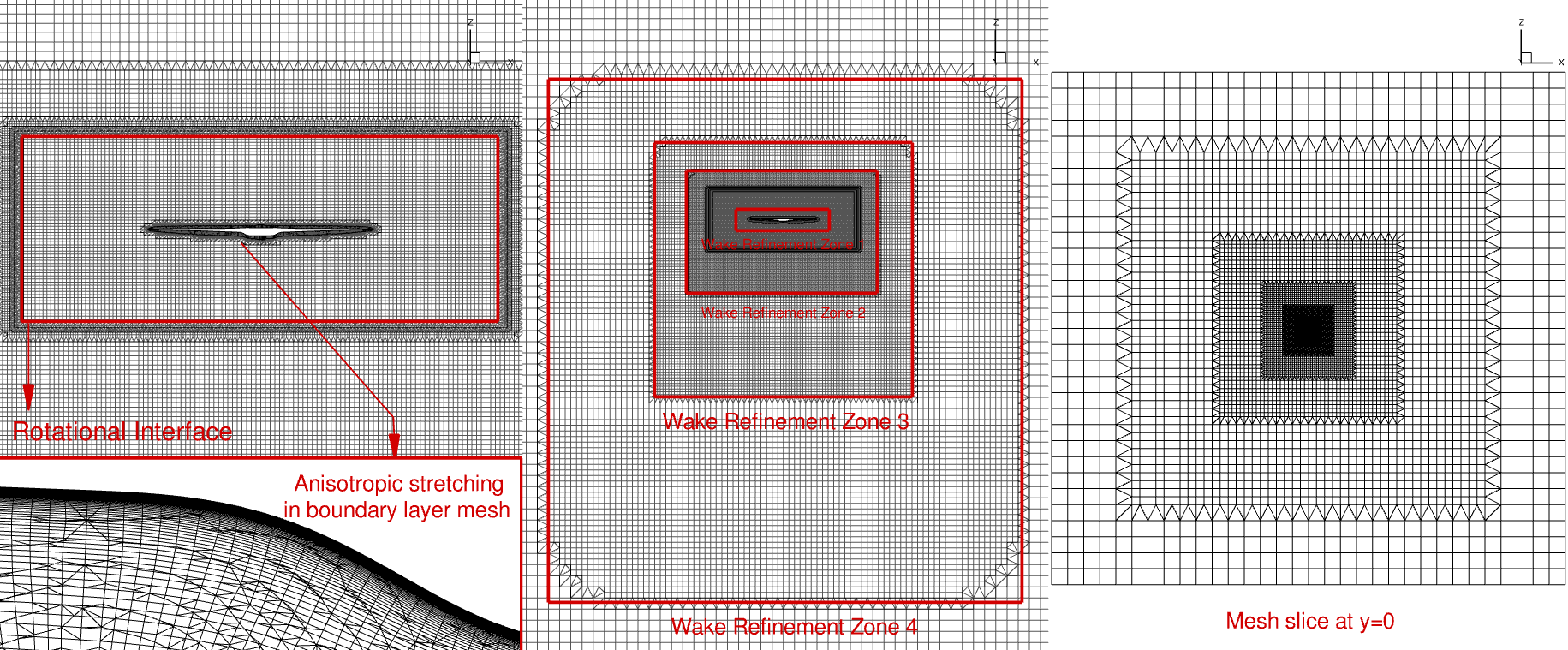
Fig. 6.12.10 Grid level 1 generated for the Mejzlik propeller.

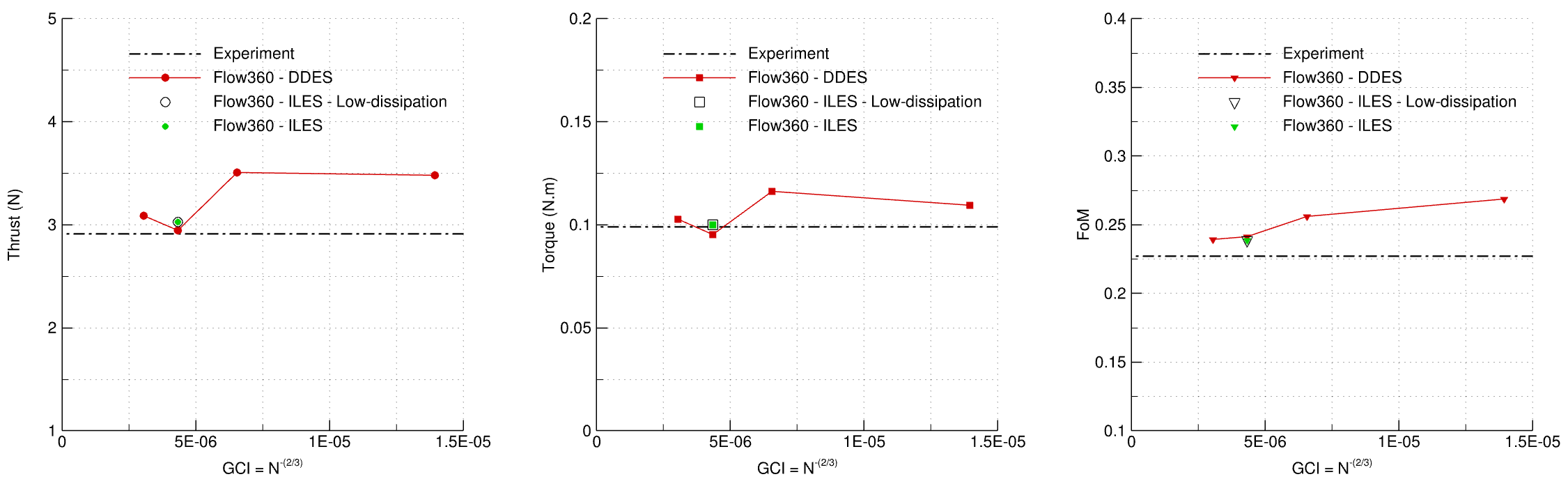
Fig. 6.12.11 Grid convergence study performed at hover mode for the Mejzlik propeller.

The results of the mesh convergence study are illustrated in Fig. 6.12.11. For the coarse grid (level 0), 240 time steps are used per revolution, which is 3/2 degrees per time step. For the medium, fine, and extra-fine grid levels, 480 time steps per revolution (3/4 degrees per revolution) are used. Fig. 6.12.11 compares outcomes across four grid levels for torque, thrust, and figure of merit (FoM) against experimental values. Concerning thrust, grid levels 2 and 3 predict it with less than a 6% error, and they forecast torque with less than a 4% error compared to experimental values. Notably, the low-dissipation simulation on grid level 2 yields the most accurate predictions, with a 4% error for thrust and a 1% error for torque compared to experimental values. grid level 2 is therefore considered sufficient.

6.12.4.3. Aerodynamic Validation

The aerodynamic loads at hover mode with a rotational speed of \(6000\) rpm are compared in Fig. 6.12.12 against experimental data provided by Baskaran et al. ⁷ and Kunz et al. ⁸. In this figure, the gray curve represents the aerodynamic load curve from the experimental data. The magenta circle corresponds to the Delayed Detached Eddy Simulation (DDES) result on grid level 2, the cyan circle represents the Implicit Large Eddy Simulation (ILES) result without the low-dissipation scheme, and the orange circle indicates the ILES result with the low-dissipation scheme both on grid level 2. Notably, the orange circle aligns more closely with experimental values for both thrust and torque at hover mode. The thrust and torque values are obtained by averaging over the last 5 revolutions after an initial 10 revolutions.

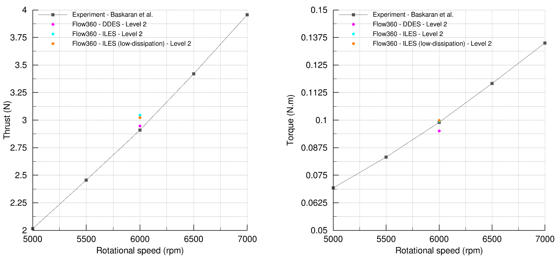
Fig. 6.12.12 Comparison of aerodynamic loads in hover mode against experimental data for ILES and DDES simulations for the Mejzlik propeller.

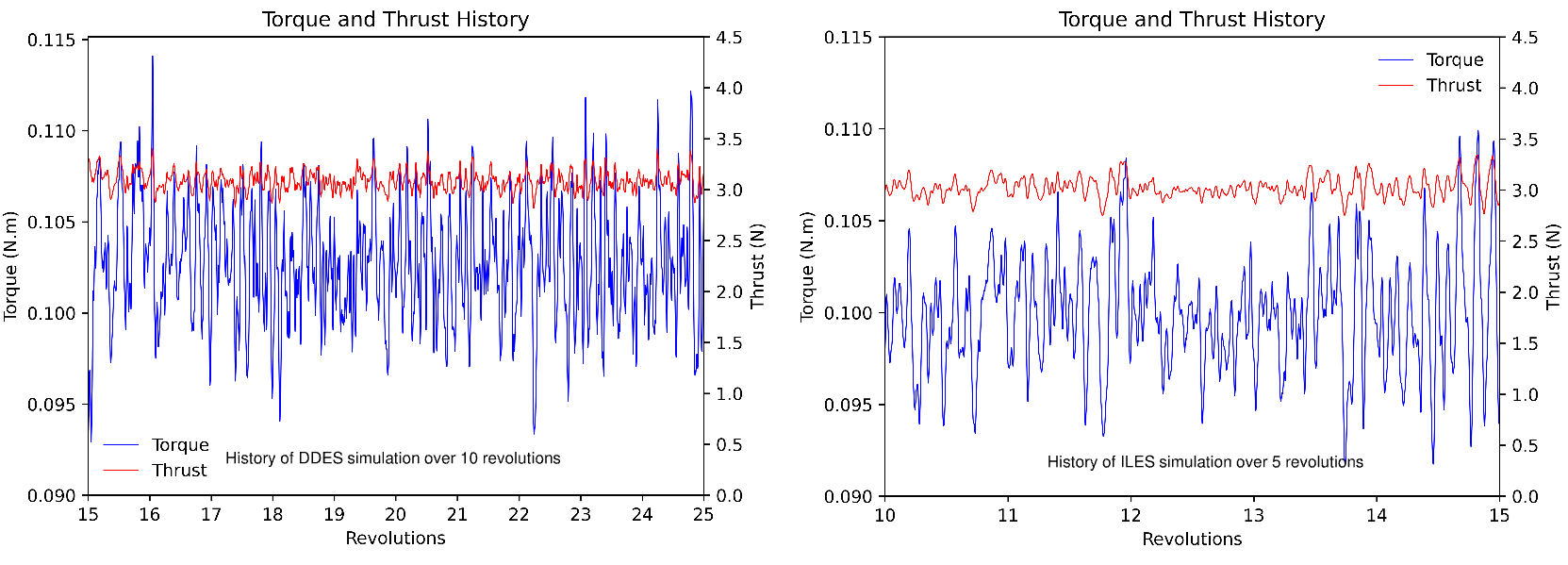
Fig. 6.12.13 Comparison of the history of aerodynamic loads in hover mode for ILES and DDES simulations for the Mejzlik propeller.

In Fig. 6.12.13, the history of aerodynamic loads are compared between Delayed Detached Eddy Simulation (DDES) and Implicit Large Eddy Simulation (ILES). For the DDES simulation, aerodynamic loads are monitored for the last 10 revolutions, while for the ILES simulation, they are monitored for the last 5 revolutions. The DDES simulation is initiated after two consecutive initial simulations. Firstly, a first-order simulation is conducted for 5 revolutions, followed by a second-order simulation for 10 revolutions. Finally, the DDES simulation begins from the solution obtained in the second-order run and lasts for 10 revolutions. The ILES simulation starts after one initial simulation. Initially, a first-order simulation is performed for 5 revolutions, and then the ILES simulation begins using the first-order solution, lasting for 10 revolutions. The aerodynamic loads are averaged over the last 5 revolutions. The comparison in this figure reveals that variations in torque and thrust after the initial 10 revolutions are similar. Therefore, it is considered that the initial 10 transient revolutions are sufficient to initiate an unsteady run and average the aerodynamic loads.

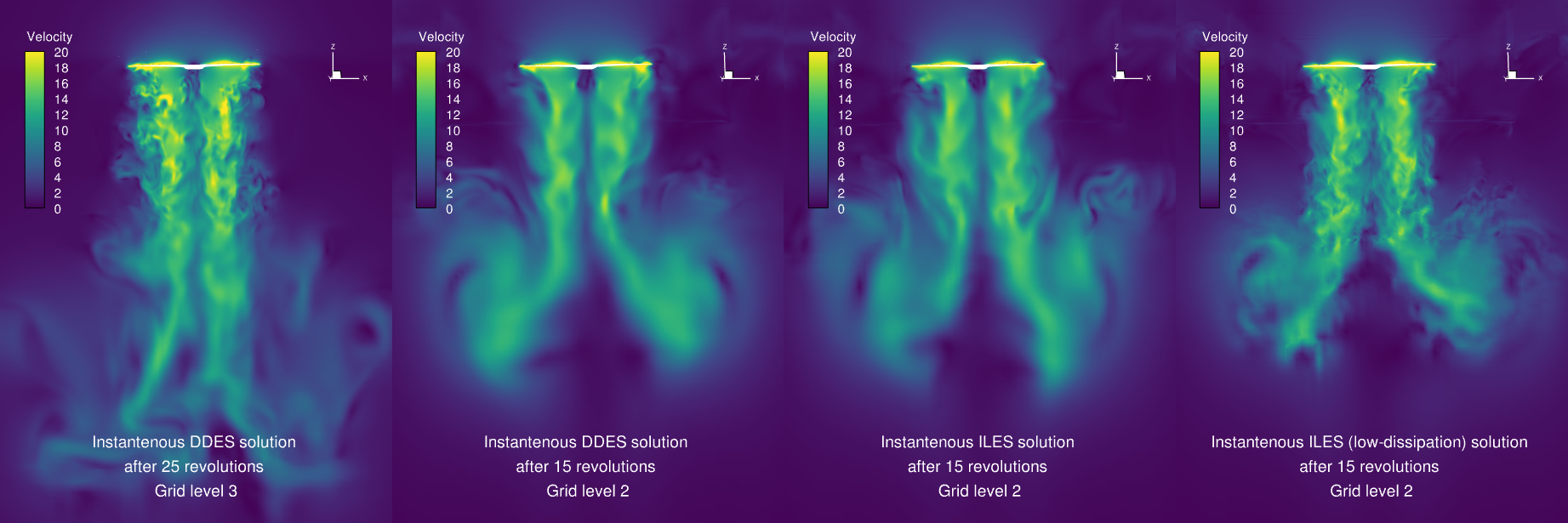
Fig. 6.12.14 Comparison of instantaneous velocity contours in hover mode for ILES and DDES simulations for the Mejzlik propeller.

In Fig. 6.12.14, instantaneous velocity contours at the middle slice are presented for both Implicit Large Eddy Simulation (ILES) and Delayed Detached Eddy Simulation (DDES) approaches. On the left side, the DDES solution on the extra fine mesh (level 3) after 25 revolutions is displayed. This represents the longest simulation on the finest mesh. Next, the DDES solution on the fine mesh (level 2) after 15 revolutions is shown. In comparison to the DDES solution on grid level 3, the vortices are more resolved in the near-field region, which is attributable to the presence of a finer mesh in the wake region. Moreover, the wake is more dissipated downstream after 2D, which stems from the mesh resolution difference between level 2 and 3. On the right side, the DDES solution on grid level 2 is compared with the ILES solution on the same grid level after 15 revolutions. The comparison of instantaneous vortical structures for both solutions on the same grid level after the same number of revolutions reveals fair similarity. Finally, the instantaneous ILES solution on grid level 2 after 15 revolutions is presented. The vortical structure in the wake region for this solution is notably similar to the DDES solution on grid level 3. The vortices are well-resolved in the wake region for the low-dissipation simulation on grid level 2. This indicates that employing the low-dissipation scheme enhances the ability to resolve turbulence in both space and time for a transient simulation. The iso-surface of the Q-criterion for different instantaneous solutions is shown in Fig. 6.12.15. It reveals some separation on the upper surface, even though this is the RANS region of the DDES, and confirms the different resolution of turbulent eddies seen earlier.

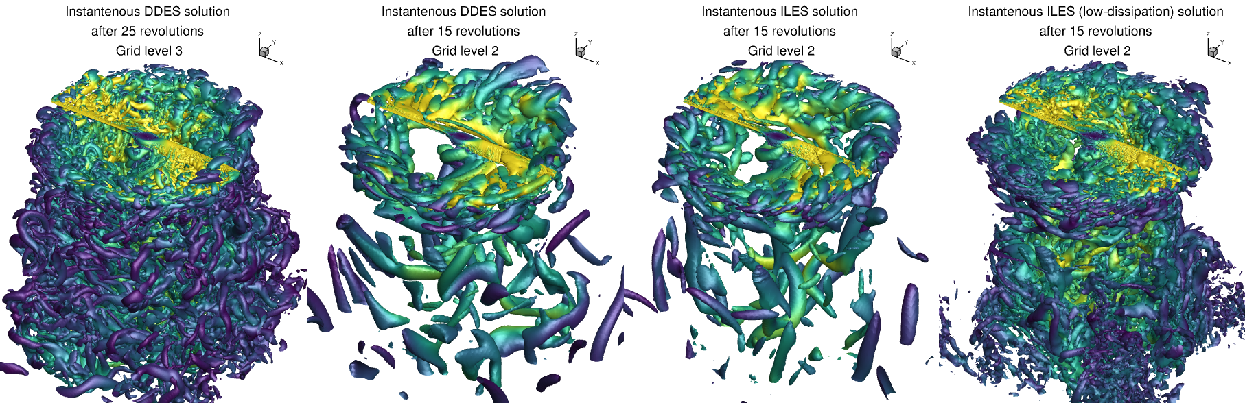
Fig. 6.12.15 Comparison of iso-surface Q-criterion in hover mode for ILES and DDES simulations for the Mejzlik propeller.

6.12.4.4. Noise Evaluation

The acoustic field is computed at 21 observation points positioned at a distance of 1.75 meters (\(7.65 \times D_{p}\)) from the propeller, aiming to obtain a wall-resolved directivity consistent with the experimental tests provided by Baskaran et al. ⁷ and Kunz et al. ⁸. The schematic representation of microphone locations is illustrated in Fig. 6.12.16. Please note that this figure is schematic and cannot be scaled. The actual locations of the microphones are at a considerable distance from the propeller for measuring far-field noise.

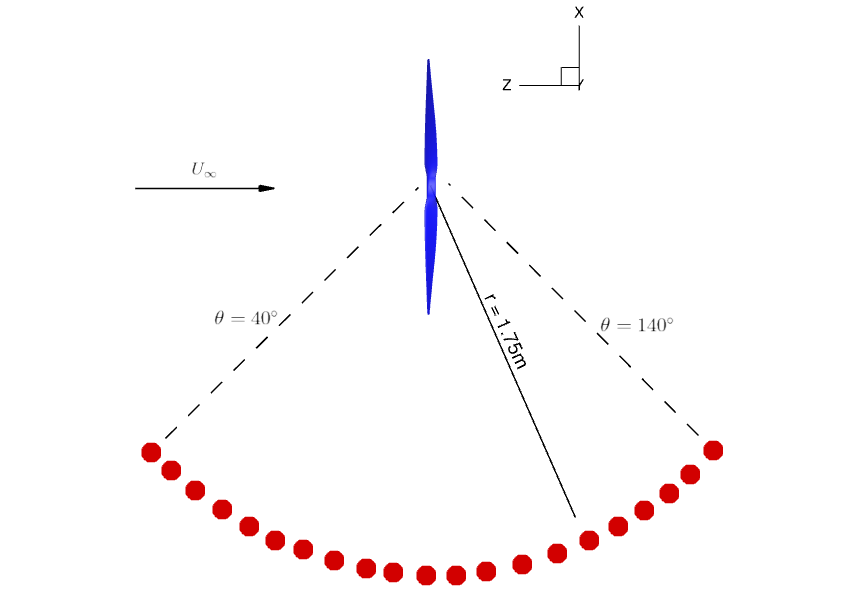
Fig. 6.12.16 Schematic locations for noise evaluation points for the Mejzlik propeller.

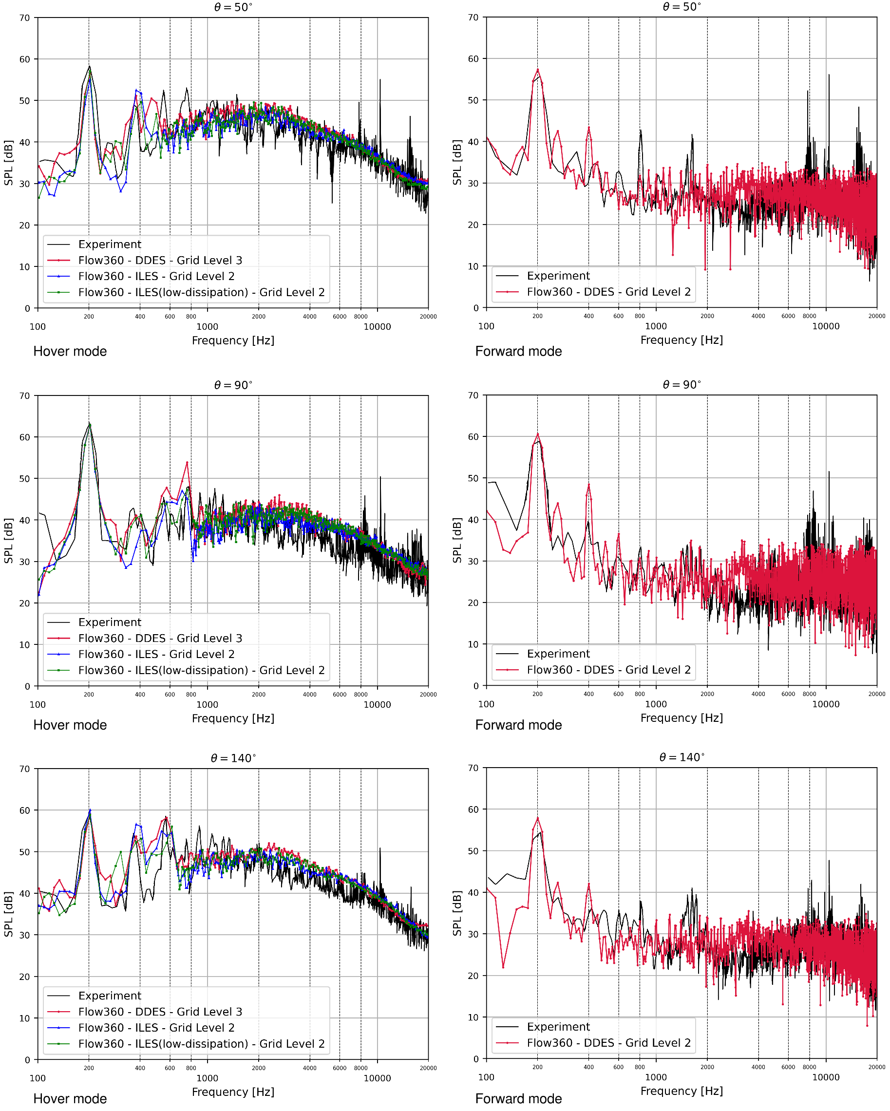
Fig. 6.12.17 Sound Pressure Level (SPL) spectra in both hover and forward modes for both DDES and ILES runs of the Mejzlik propeller.

The sound pressure level (SPL) spectrum for the DDES run on grid level 3 and ILES runs on grid level 2 is shown in Fig. 6.12.17 at microphone locations at \(\theta=\) 50, 90, and 140 degrees, representing upstream, in-plane, and downstream observers. As observed in this figure, the simulations accurately predict the tonal noise, with all three simulations capturing the peak and even the width of the tonal noise effectively. The agreement between the experimental and numerical results is notably good, indicating a reliable prediction of tonal noise characteristics by the simulations. In forward flight, there is a slight over-prediction of the tonal noise. The broadband noise is much lower, as a result of the vortices moving away from the blade much more rapidly, and/or of the blade having a lower lift coefficient and less separation.

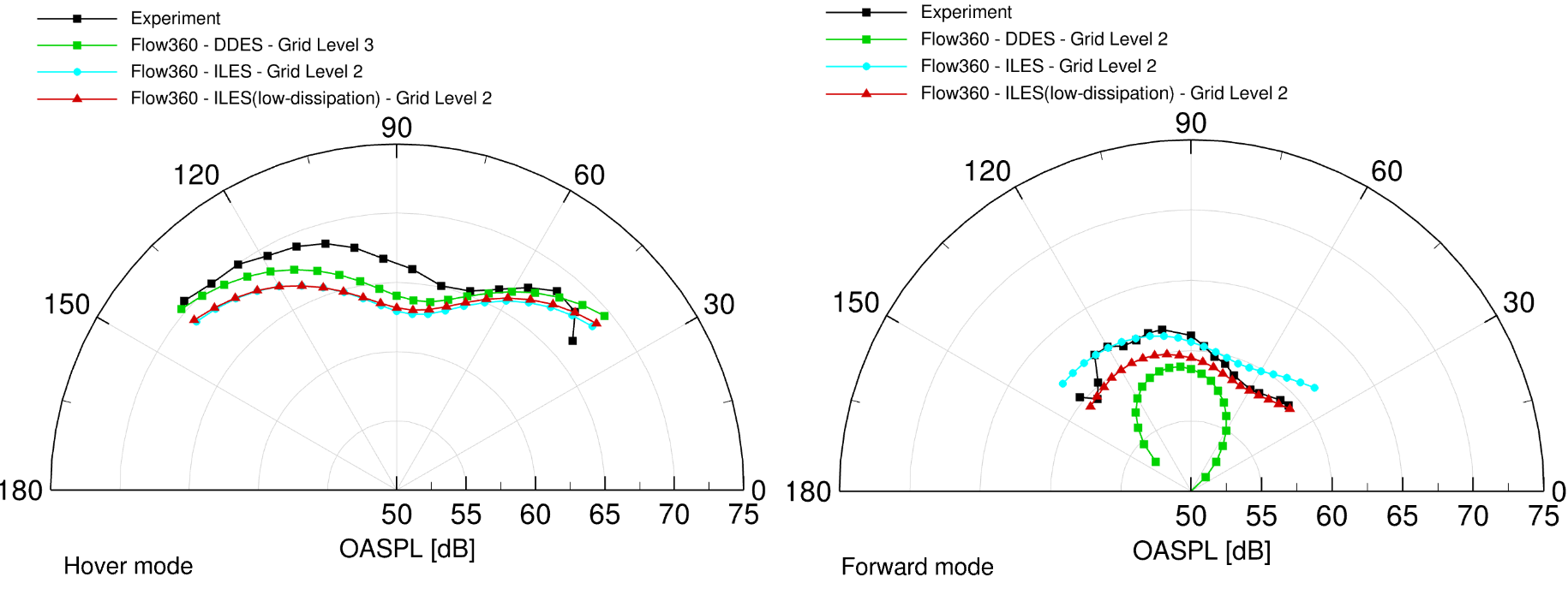
Fig. 6.12.18 Overall Sound Pressure Level (OASPL) in both hover and forward modes for both DDES and ILES runs of the Mejzlik propeller.

The Overall Sound Pressure Level (OASPL) for both hover and forward modes in both Delayed Detached Eddy Simulation (DDES) and Implicit Large Eddy Simulation (ILES) simulations is presented in Fig. 6.12.18. In hover mode, the OASPL from the DDES simulation on grid level 3 closely aligns with experimental results. Additionally, the ILES simulation with the low-dissipation scheme also exhibits a strong agreement with experimental OASPL. In the forward mode, the ILES simulation with the low-dissipation scheme accurately predicts both the OASPL values and their directional characteristics compared to the experimental data. This is partly thanks to compensating errors in the spectrum. The iso-surface Q-criterion surface plot in forward mode for both DDES and ILES simulations on grid level 2 is displayed in Fig. 6.12.19. Some separation on the upper blade surface is seen with ILES, and probably linked to the lack of turbulence model. This visualization highlights the improved resolution of vortical structures in the ILES simulation with the low-dissipation scheme on the same grid level. It also shows that the DDES has no separation on the blade, unlike the ILES which lacks a fine-enough grid to resolve the boundary-layer turbulence. Neither simulation resolves turbulence inside the tip vortex, a sign that there is much room for further grid refinement.

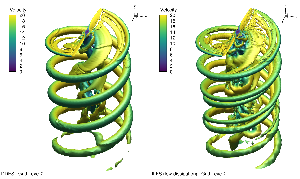
Fig. 6.12.19 Iso-surface Q-criterion plot in forward mode on grid level 2 for both DDES and ILES runs of the Mejzlik propeller.

⁽¹⁾ Jacob, M.C., Boudet, J., Casalino, D. and Michard, M., 2005. A rod-airfoil experiment as a benchmark for broadband noise modeling. Theoretical and Computational Fluid Dynamics, 19, pp.171-196.

⁽²⁾ Casalino, D., Jacob, M. and Roger, M., 2003. Prediction of rod-airfoil interaction noise using the Ffowcs-Williams-Hawkings analogy. AIAA journal, 41(2), pp.182-191.

⁽³⁾ Peth, S., Seo, J.H., Moon, Y.J., Jacob, M.C. and Thiele, F., 2006. Computation of Aerodynamic Noise from Rod Wake–Airfoil Interactions, Eur. In Conf. Comput. Fluid Dyn., The Netherlands.

⁽⁴⁾ Galdeano, S., Barré, S. and Réau, N., 2010. Noise radiated by a rod-airfoil configuration using DES and the Ffowcs-Williams & Hawkings’ analogy. In 16th AIAA/CEAS aeroacoustics conference (p. 3702).

⁽⁵⁾ Giret, J.C., Sengissen, A., Moreau, S., Sanjosé, M. and Jouhaud, J.C., 2012. Prediction of the sound generated by a rod-airfoil configuration using a compressible unstructured LES solver and a FW-H analogy. In 18th AIAA/CEAS Aeroacoustics Conference (33rd AIAA Aeroacoustics Conference) (p. 2058).

⁽⁶⁾ Travin, A., Shur, M., Strelets, M. and Spalart, P., 2000. Detached-eddy simulations past a circular cylinder. Flow, turbulence and combustion, 63(1-4), pp.293-313.

⁽⁷⁾ Baskaran, K., Jamaluddin, N.S., Celik, A., Rezgui, D. and Azarpeyvand, M., 2022. Aerodynamic and aeroacoustic characteristics of propellers with different blade numbers. In 28th AIAA/CEAS Aeroacoustics 2022 Conference (p. 3108).

⁽⁸⁾ Kunz, F., Zhou, B.Y., Pullin, S.F., Azarpeyvand, M., Galimberti, L., Morelli, M. and Guardone, A., 2023. High-Fidelity Propeller Broadband Noise Prediction using SU2. In AIAA AVIATION 2023 Forum (p. 4185).

6.12.5. Conclusions

The case study provides several recommendations for aeroacoustics and noise simulation:

1. Extruded Configuration and Spanwise Length:

   • For extruded configurations, it is advisable to set the spanwise length close to or larger than the spanwise coherence length to effectively resolve flow structures. This would be difficult for the coherence length at the vortex-shedding frequency.

   • Using periodicity is recommended, but when employing CFD with the FWH analogy, it may be necessary to distribute observer locations in the span direction to account for length effects. This is not an issue with real-world systems wich are finite in all directions.

2. Reynolds Number Considerations:

   • For low Reynolds number flow regimes with transitional unsteady flow, Implicit Large-Eddy Simulation (LES) is recommended, because the RANS modeling in DDES treats the boundary layer as turbulent everywhere.

   • For high Reynolds number flows, Delayed Detached Eddy Simulation (DDES) is recommended because RANS modeling is appropriate.

3. Assurance of CFD Simulation Quality:

   • It is crucial to ensure that the CFD simulation used for aeroacoustic analysis is of high quality and effectively captures unsteady loads.

4. Mesh Resolution:

   • Adequate mesh resolution on solid bodies, near-field and wake regions, and around noise sources is essential for the accurate capture of Sound Pressure Level (SPL) spectra and Overall Sound Pressure Level (OASPL).

   • Performing a mesh convergence study is recommended to achieve optimal mesh resolution with desirable accuracy and computing cost.

5. Low-Dissipation Scheme:

   • The use of a low-dissipation scheme is advised as it enhances turbulence resolution in both time and space, particularly on relatively coarser meshes, resulting in more accurate SPL spectra and OASPL.

6. Validation of Flow360 Solver:

   • The Flow360 solver has been validated against experimental data and other scale-resolving simulations for two test cases: laminar separation flow over the rod-airfoil configuration and a two-bladed propeller.

   • Good agreement is observed for noise spectra and OASPL when compared to experimental data.

These recommendations highlight key considerations and best practices for aeroacoustic analysis using Flow360.