6.4. Transition Modeling

6.4.1. Introduction

The main purpose of this case study is verification and validation of the transition model implemented within the Flow360 solver. Additionally, mesh sensitivity effects are examined to provide best-practice guidelines for using the transition modelling capability in the Flow360 solver. Transition modelling is of key importance when a significant portion of the boundary layer remains laminar and the fully-turbulent modelling assumption is no longer valid. Transition to turbulence occurs at low Reynolds numbers (order of \(10^5\) and lower), and is important to capture in many aerospace applications such as turbomachinary, rotorcraft and fixed-wing aircraft. The model implemented in the Flow360 solver is based on the the SA-AFT (Amplification Factor Transport) 2019b model developed by Coder with details of the model presented on the NASA Turbulence Modelling Resource (TMR) Website. The AFT model is also compatible with the \(k-\omega\) SST turbulence model. The AFT model is based on linear stability theory, which aims to track the growth of pressure/velocity instabilities in the boundary layer. This approach more directly aligns with the physics involved with the transition process as compared to correlation based models. The model is coupled with the Spalart-Allmaras (SA) turbulence model through a modification of the \(f_{t2}\) term with two additional transport equations solved, one for modified intermittency and one for the approximate envelope amplification factor.

The present case study targets two cases, a canonical zero-pressure gradient flat plate and flow past an NLF(1)-0416 airfoil, designed to maintain laminar flow in aerospace applications. Firstly, the zero-pressure gradient flat plate case is demonstrated with transition based on the NASA TMR Flat Plate Validation Case. The cases from the 1st Transition Prediction Workshop are not used here, as transition models based on the AFT framework are not tailored to cases with high freestream turbulent eddy viscosity ratio’s, which target bypass transition conditions. An assessment of grid element type is made to examine mesh sensitivity effects. Following, detailed comparisons are made with the results presented by Coder using the SA-AFT model in OVERFLOW. The primary objective of this case is verification of the SA-AFT model in the Flow360 solver, as well as preliminary validation and examination of mesh sensitivity effects.

Next, results are presented for the NLF(1)-0416 airfoil. A detailed mesh sensitivity study is presented that includes an examination of 2D vs pseudo-3D effects, grid element type and topology, with the aims to provide best-practices when using the Flow360 solver. A simulation is also performed for a 3D configuration to confirm the validity of the pseudo-3D results. Then, results from the mesh convergence study are compared with data from Coder using the SA-AFT model in OVERFLOW and Venkatachari et al. who presented data using the \(\gamma- Re_\theta\) transition model in OVERFLOW and FUN3D. Additionally, results obtained for the full angle of attack sweep are compared with experimental data and OVERFLOW data from Coder with the aim to validate the Flow360 transition model.

6.4.2. Flat Plate Case

6.4.2.1. Simulation Setup

The flat plate case is based on the model verification case available on the NASA TMR website. The freestream Mach number is equal to 0.2 with the Reynolds number per unit length equal to 5 million. The boundary conditions applied are based on the Flat Plate TMR Case as shown in Fig. 6.4.1. A sample flow configuration file is provided here.

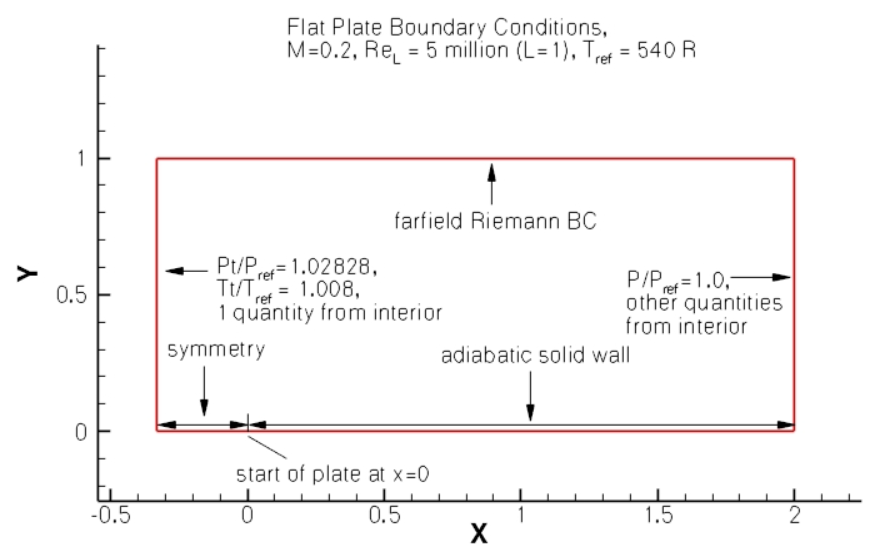
Fig. 6.4.1 Summary of boundary conditions and operating conditions for the zero pressure gradient flat plate case.

The simulations are performed using SA-AFT model with an \(N_{crit}\) value of 10.3 for consistency with the study of Coder and data from experiments for the skin friction coefficient. The grids were taken from the NASA TMR Flat Plate grids download page with five grid levels available ranging from 35 by 25 to 545 by 385 in the x-z plane with 2 nodes in the spanwise direction, as shown in Table 6.4.1.

Table 6.4.1 Grid dimensions for the flat plate case mesh convergence study.

Level	Number of nodes (x by z by y)
L1	35 x 25 x 2
L2	69 x 49 x 2
L3	137 x 97 x 2
L4	273 x 193 x 2
L5	545 x 385 x 2

The five grid levels are used to conduct a mesh convergence study and assess what impact the mesh refinement has on the transition location. Additionally, grids with different element types are also compared to perform an initial mesh sensitivity study. The baseline hexahedral grid was split into prisms to give a triangulated grid on the x-z plane. Note as the grid has only 2 nodes across, quadrilaterals are still used in the spanwise direction and hence are on the surface of the flat plate. A comparison of the mid-span (x-z) plane is shown in Fig. 6.4.2.

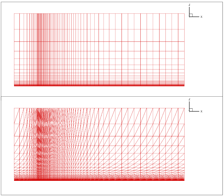
Fig. 6.4.2 Comparison of the quad (top) and tri (bottom) grids for the flat plate case.

6.4.2.2. Numerical Results

The mesh convergence for the flat plate case for quad and tri meshes is analysed in terms of the skin friction distribution shown in Fig. 6.4.3.

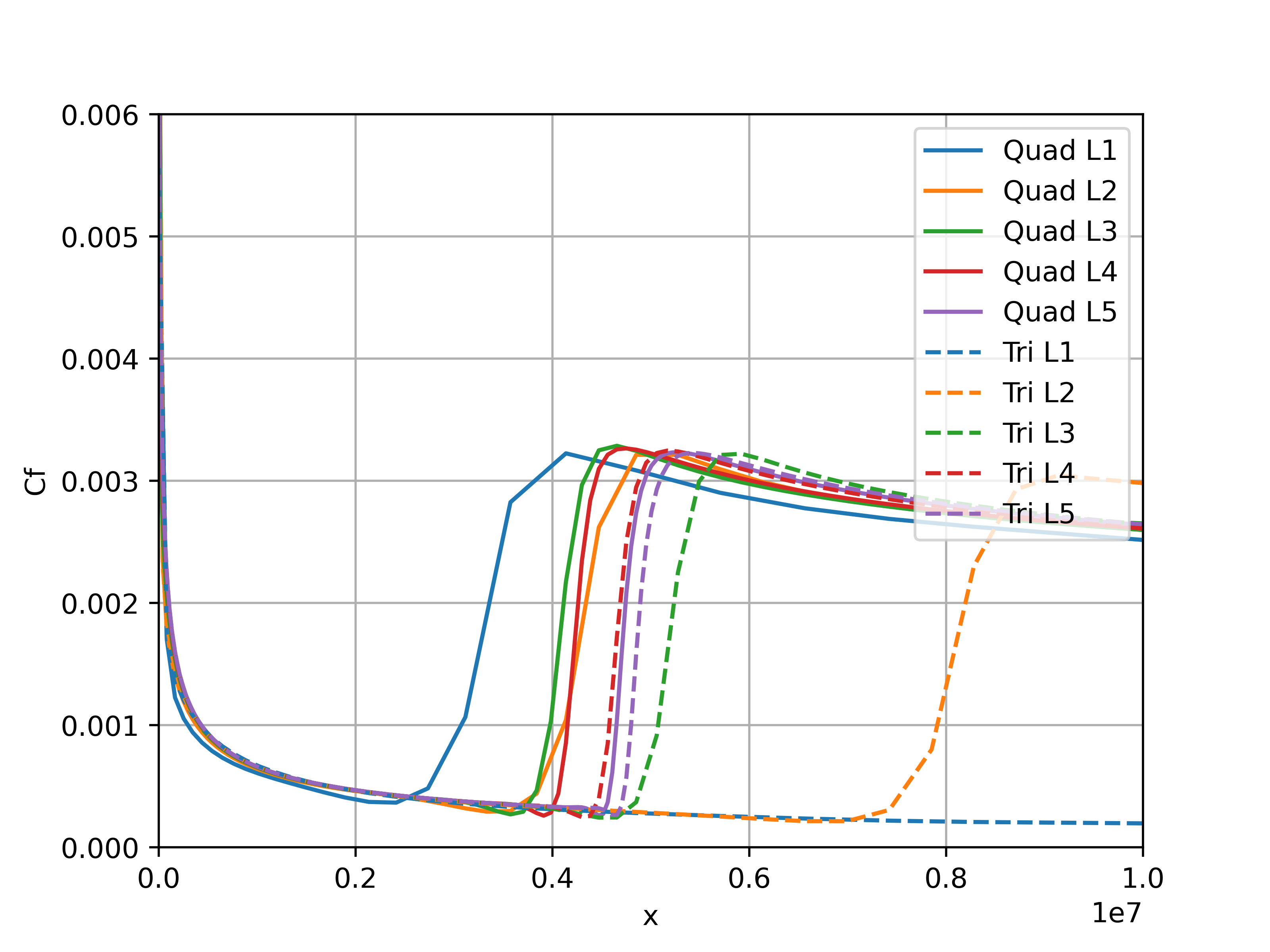
Fig. 6.4.3 Comparison of skin friction distribution grid convergence for quad and tri meshes for the flat plate case.

The grid convergence of the skin friction distribution on the flat plate shows that the result is not fully grid converged. The behaviour of the meshes with quads is different than the meshes with tri elements. For the coarsest tri mesh, no transition is detected and as the grid is refined, the transition location moves upstream, apart for the finest two levels where the transition location moves downstream. For the quad meshes, the convergence is highly non-linear. Initially the transition location moves downstream, before moving upstream for grid level 3, and then moving downstream for levels 4 and 5. The transition location for the finest two meshes (level 5) is very close for both quad and tri meshes. The tri meshes appear to be more dissipative for coarser meshes, however, have a lower sensitivity to transition location for finer meshes when compared to the quad meshes. Next the skin friction distributions are compared for the two finest grids with data from OVERFLOW and experimental data from Schubauer-Klebanoff, shown in Fig. 6.4.4.

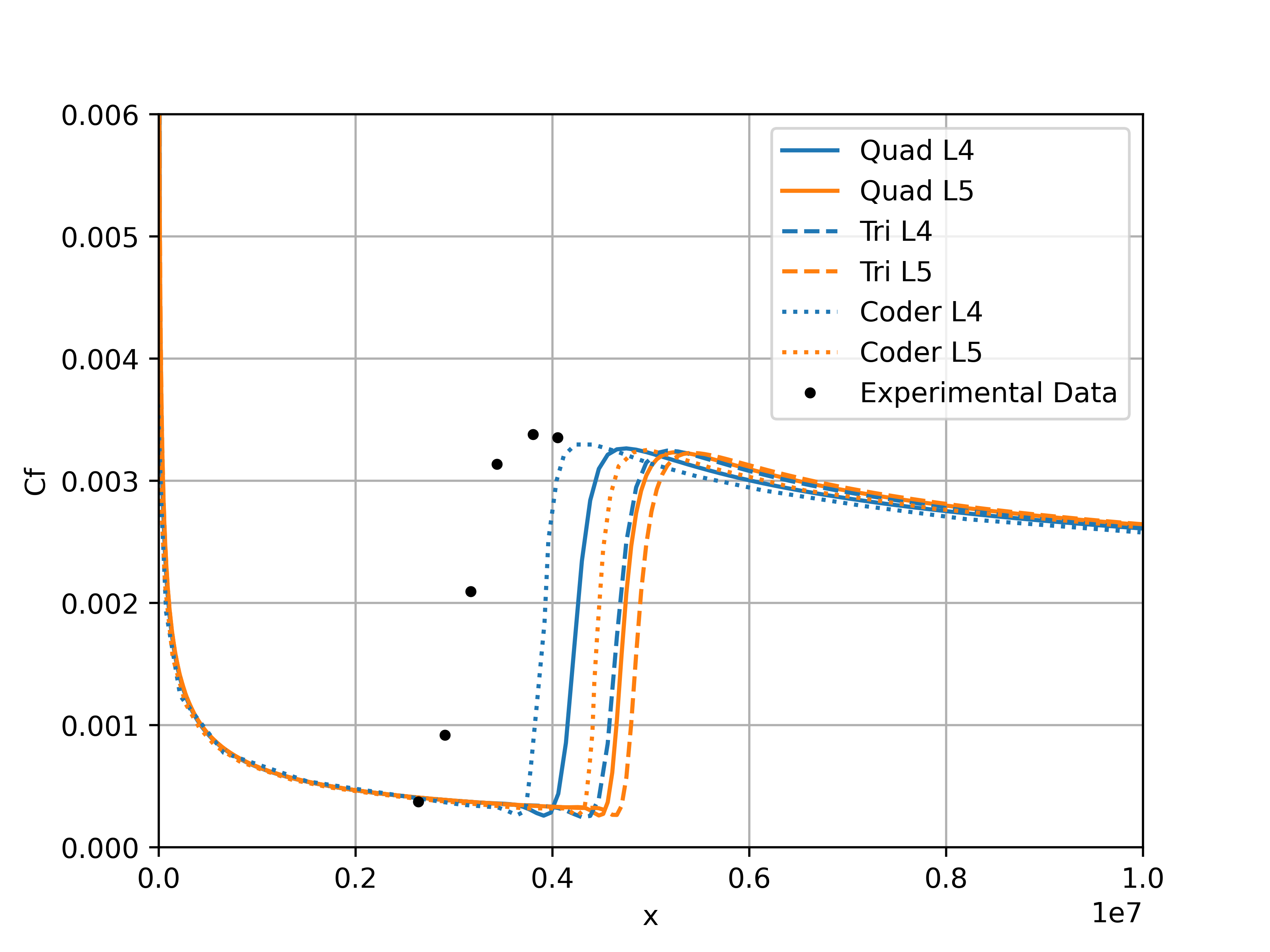
Fig. 6.4.4 Comparison of skin friction distribution for the two finest grids with OVERFLOW and experimental data for the flat plate case.

The skin friction distributions indicate that both Flow360 and OVERFLOW predict a transition location that is further downstream when compared to experiments. Flow360 predicts a transition location slightly further downstream than OVERFLOW, however, the difference reduces as the grid is refined. Finer grids would be required to perform a complete verification of the transition model in Flow360. The grid convergence for the finest two grids shows the same pattern between Flow360 and OVERFLOW, as the L5 grid moves further away from experiments than the L4 grid. The lack of grid convergence for the flat plate was due to the intermittency equation and its coupling with the SA turbulence model, according to Coder. Another potential aspect is the fact that the transition location may be highly sensitive to numerics with no presence of a pressure gradient. To further examine the differences between Flow360 and OVERFLOW, the volumetric modified intermittency and amplification factor contours are extracted from the solutions, shown in Fig. 6.4.5 - Fig. 6.4.6.

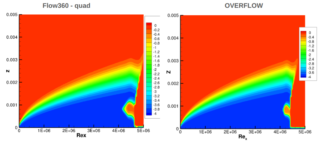
Fig. 6.4.5 Comparison of the modified intermittency contours between Flow360 and OVERFLOW for flat plate case on the finest grid.

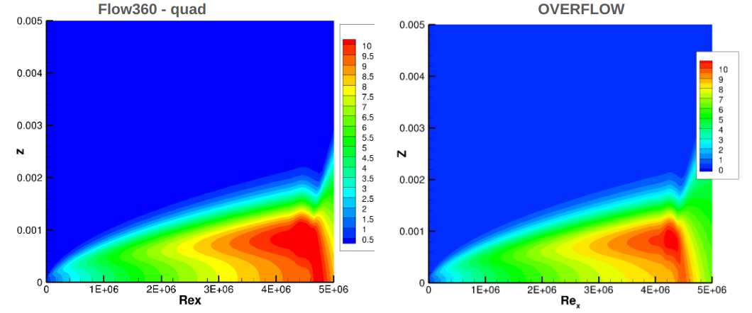
Fig. 6.4.6 Comparison of the amplification factor contours between Flow360 and OVERFLOW for flat plate case on the finest grid.

The contours of the modified intermittency show a high degree of consistency between Flow360 and OVERFLOW. The primary difference is the prediction of the transition location slightly further downstream for the Flow360 solution. The Flow360 prediction also predicts a slightly larger turbulent spot ahead of the transition location. The amplification factor contours also show good correlation, although slightly higher magnitudes are observed in the Flow360 solutions. This is primarily due to the prediction of transition further downstream, hence the instabilities have a longer distance to grow. The tri and quad solutions were consistent with differences mainly attributed to the different transition location.

6.4.3. NLF(1)-0416 Airfoil Case

The second case that was analysed was the NLF(1)-0416 airfoil case, which is more applicable to aerospace applications. Firstly, the simulation setup is presented including a number of grid families generated to examine mesh sensitivity effects. The first part of the results focuses on an analysis of grid convergence for each grid family is performed, before further analysing the effect of 2D vs pseudo-3D solutions and the effect of element types. In the final part of the results, the solutions are compared with other solvers and experimental data.

6.4.3.1. Simulation Setup

The NLF(1)-0416 airfoil case is based on Case 2 of the 1st Transition Prediction Workshop. The flow conditions are a Mach number of 0.1, Reynolds number of 4 million based on the chord length and freestream \(N_{crit}\) value of 7.2. For this case, the SA-AFT transition model is also used. A sample flow configuration file is provided here. The case involves a mesh convergence study at an angle of attack of 0 and 5 degrees as well as a full angle of attack sweep.

6.4.3.1.1. Grid Families

As mesh sensitivity effects are of interest to provide best-practice guidelines, multiple grid families are generated for the mesh convergence study. The primary aims are to establish whether 2D simulations are valid when compared to pseudo-3D and 3D simulations for transition predictions, and what element types should be used on the surface and in the volume mesh to reduce grid sensitivity effects. For this purpose, the following grid families are generated, with further details provided below:

1. Family 1: 2D baseline hexahedral grids (6 levels) provided on the 1st Transition Prediction Workshop Page . These were modified to only include 2 nodes (rather than 3) in the spanwise direction for pure 2D solutions.

2. Family 2: Pseudo-3D hexahedral grids. Modified baseline hexahedral grids to include 20 nodes in the spanwise direction, generated through spanwise extrusion

3. Family 3: 2D triangulated baseline grids. The cells on the symmetry planes were triangulated, similarly as for the flat plate case study. This leads to quadrilateral cells on the airfoil surface with prism cells in the volume, with 2 nodes in the spanwise direction.

4. Family 4: Pseudo-3D triangulated baseline grids. Modified 2D triangulated baseline grids (Family 3) to include 20 nodes in the spanwise direction, generated through spanwise extrusion

5. Family 5: Pseudo-3D triangulated surface baseline grids. These were generated manually by applying the same number of nodes and LE/TE spacings as for the Family 2 grids and generating a triangulated structured surface grid, and then generating an unstructured prism-tet volume grid with settings extracted from the Family 1 grids. These grids have 20 nodes in the spanwise direction (over 1 chord length).

6. Family 6: Pseudo-3D triangulated surface baseline grids with varying number of spanwise nodes. This family includes the ultra-fine grid (Level 6) settings from Family 5 with spanwise node values of 20, 40 and 80.

7. Family 7: Pseudo-3D fully unstructured grids. These grids were generated using the automated meshing workflow of Flow360. The inputs to the surface and volume mesher were extracted from the Family 1 grids to ensure a high degree of consistency between different grid families. To minimize the node count, the span is reduced from 1 chord to 0.04 chord.

6.4.3.1.2. Grid Levels

Families 1 to 4 are all based on the baseline C-topology committee grids. The baseline committee extracted grid properties (approximated) are shown in Table 6.4.2.

Table 6.4.2 Approximate extracted grid properties for the NLF(1)-0416 case mesh convergence study. \(\Delta S\) = Spacing on the surface, \(\Delta Y\) = First cell height in the volume, GR = Growth Rate, C = Chordwise, N = Normal, W = Wake Cut (downstream of TE).

Level	LE \(\Delta S\)	TE \(\Delta S\)	Max \(\Delta S\)	Wall \(\Delta Y\)	Vol GR.	Num. nodes (C by N by W)
L1	0.0019	0.0011	0.012	7e-06	1.45	353 x 49 x 49
L2	0.00125	0.0007	0.0076	4.5e-06	1.28	529 x 73 x 73
L3	0.0009	0.0005	0.0056	3.2e-06	1.20	705 x 97 x 97
L4	0.0006	0.00033	0.0038	2.0e-06	1.13	1057 x 145 x 145
L5	0.00045	0.00025	0.0028	1.5e-06	1.1	1409 x 193 x 193
L6	0.00032	0.00016	0.0019	1.0e-06	1.065	2113 x 289 x 289

Families 1 and 2 have hexahedrals in the volume grid, whereas Families 3 and 4 have prisms in the volume grid, with all four families having quadrilateral elements on the surface. Families 5, 6 and 7 have triangular elements on the surface with prisms in the volume grid, and were generated from an ESP model of the NLF(1)-0416 airfoil with a blunt trailing edge. The main difference between Families 5, 6 and 7 is the fact that the automated meshing workflow does not guarantee an equal spacing in the spanwise direction on the surface. Grids in Family 7 will therefore, have more nodes in the spanwise direction near the leading and trailing edges than in the airfoil midsection, primarily due to the constraint on the cell aspect ratio of 25 (for this reason the span was reduced from 1 to 0.04), whereas grids in Family 5 and 6 have a uniform spanwise spacing along the airfoil. The settings for the surface meshes in Family 7 and the volume meshes in Families 5-7 were exactly the same as shown in the table above. The total number of nodes for Families 1-7 are shown in Table 6.4.3. Note that L6 in Family 5 is the same grid as L1 in Family 6 (20 nodes in spanwise direction).

Table 6.4.3 Number of nodes for the various grid levels in Families 1 to 7.

Level	F1, F3	F2, F4	F5	F6	F7
L1	34,496	362,208	177,179	3,977,171	550,640
L2	77,088	809,424	331,070	7,921,793	1,002,309
L3	136,576	1,434,048	542,461	15,896,483	1,717,135
L4	306,240	3,215,520	1,117,852		2,960,525
L5	543,488	5,706,264	1,837,248		4,901,349
L6	1,220,736	12,817,728	3,977,171		14,053,258

As can be seen from the table above, the pseudo-3D cases require significantly more grid points than the pure 2D cases. The triangular surface grids (Families 5-7) require fewer points for a given grid level primarily due to the fact that they were generated using an unstructured solver, not spanwise extrusion, hence the number of spanwise nodes in the volume typically reduces closer to the farfield. Grid Family 6 contains an increase in spanwise nodes up to 80 for level 3. A grid of 40 nodes in the spanwise direction was also generated for the grid Family 2 but not shown in the Table (25,025,088 nodes). Grid Family 7 contains significantly more nodes than Family 5 even though the spanwise spacing was reduced to 0.04, which is primarily due to the aspect ratio constraint of 25 for these grids. In the mesh convergence study, the metric used along the x-axis is 1 over the number of surface nodes. As the number of chordwise nodes will be more important than the number of spanwise nodes, the number of surface nodes is divided by 20 for pseudo-3D cases (to align Families 1 and 2, 3 and 4 on the x-axis).

6.4.3.1.3. Grid Comparisons

The surface grids and cuts through the mid-plane of the volume mesh are presented for Level 2 grids of different Families in Fig. 6.4.7 and Fig. 6.4.8. The Family 6 grids are not shown here, as these used the L6 grids of Family 5 with a variation in the number of spanwise nodes.

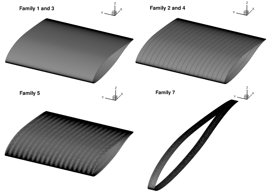
Fig. 6.4.7 Comparison of the surface grids for different grid families.

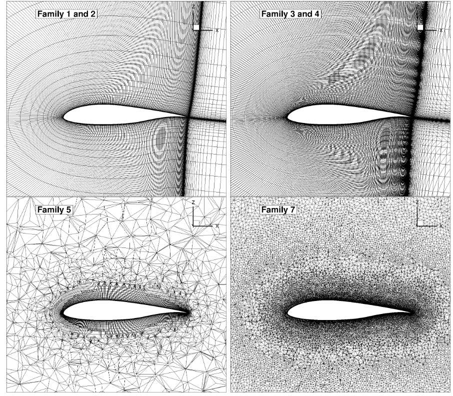
Fig. 6.4.8 Comparison of the volume grids for different grid families (slice through mid-span y=-0.5).

It is clear from the volume grid visualizations that the grid Family 7 is a much higher quality unstructured grid than grid Family 5 though a higher number of nodes was used. This is primarily due to the fact the grid Family 5 has 20 nodes across a spanwise length of 1 chord, leading to high aspect ratio cells. Furthermore, there is little control over the volume grid in the mid section of the airfoil.

Finally, a single grid was also generated for the 3D wing geometry using an aspect ratio of 20 (semi-span of 10 chords). The grid was generated using the automated meshing workflow of Flow360. The cell aspect ratio constraint of 25 was loosened to 100 to reduce the number of nodes in the grid. The surface settings were based on the L2 grid properties for the surface and the L6 grid properties for the volume. The primary purpose of the 3D wing simulation is to ensure that similar transition locations were obtained as for the pseudo-3D cases away from the root and tip of the wing. To perform these simulations, the user defined dynamics feature was switched on with the wing CL trimmed to the values obtained for the L6 grid of grid Family 1. This is done by automatically adjusting the angle of attack, according to an update law specified by the user to match the specified lift coefficient. A section of the surface grid as well as a slice at mid-span of the volume grid for the 3D wing configuration is shown in Fig. 6.4.9

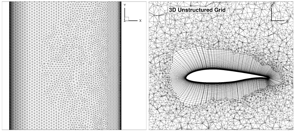
Fig. 6.4.9 A section of the surface grid along with the volume grid (slice through mid-span y=-0.5) for the 3D wing configuration.

6.4.3.2. Grid Convergence Study

Firstly, the convergence of the integrated loads with mesh refinement is extracted at two angles of attack of 0 and 5 degrees shown in Fig. 6.4.10-Fig. 6.4.13. Note that the number of surface nodes was divided by 20 for all pseudo-3D cases to ensure a fair comparison (number of nodes in spanwise direction less important than in chordwise direction).

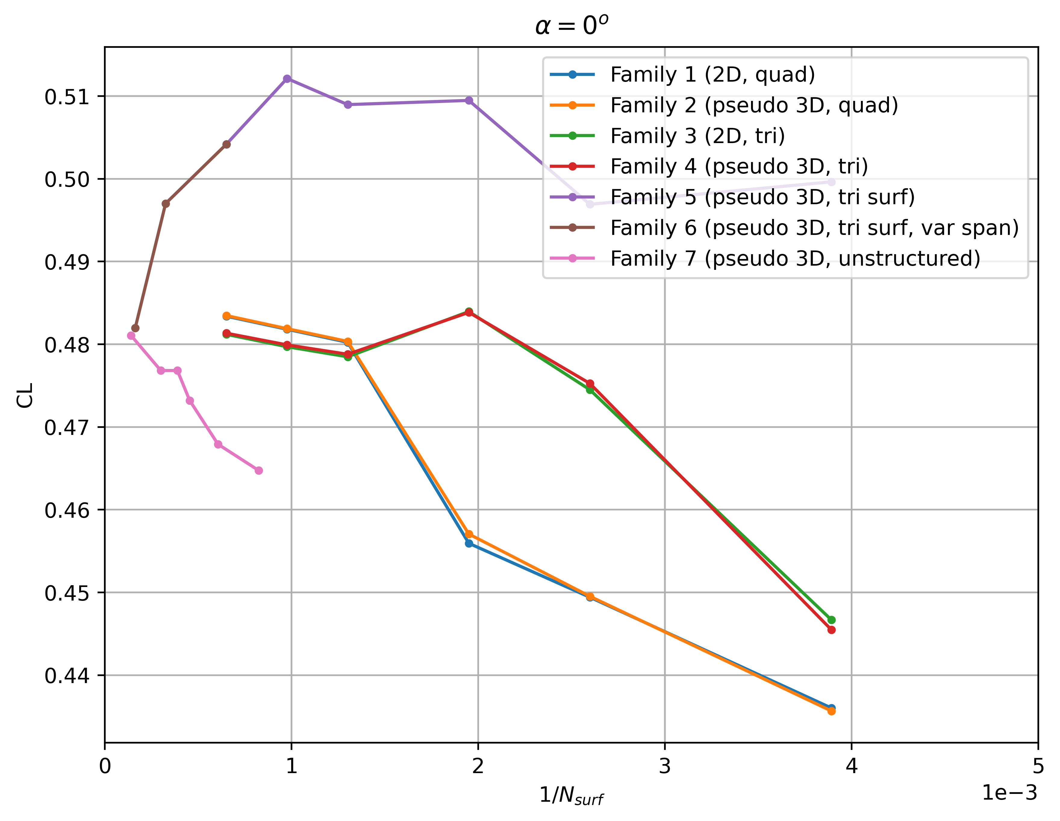
Fig. 6.4.10 Convergence of the lift coefficient with mesh refinement at \(\alpha = 0^o\) for 7 different grid families.

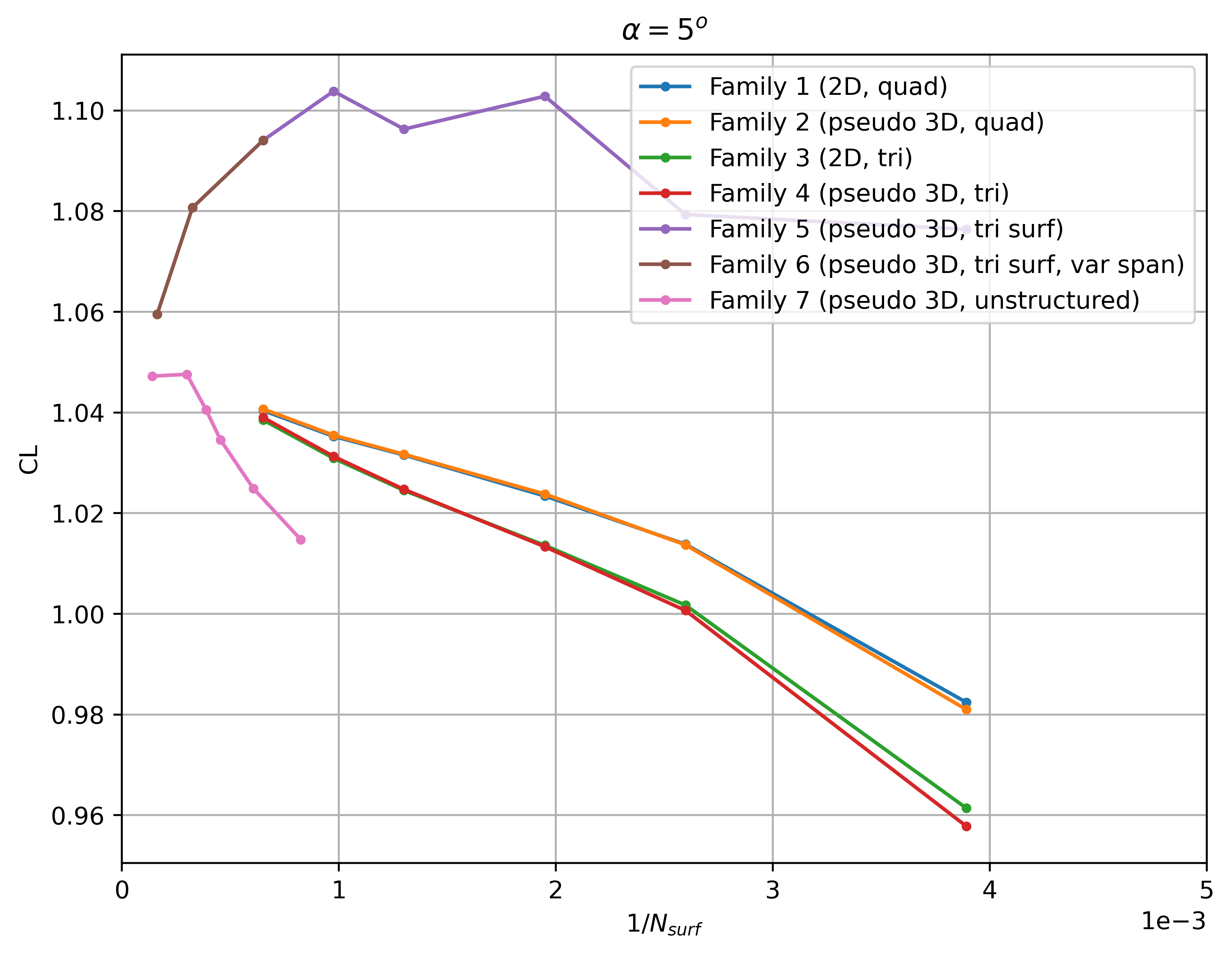
Fig. 6.4.11 Convergence of the lift coefficient with mesh refinement at \(\alpha = 5^o\) for 7 different grid families.

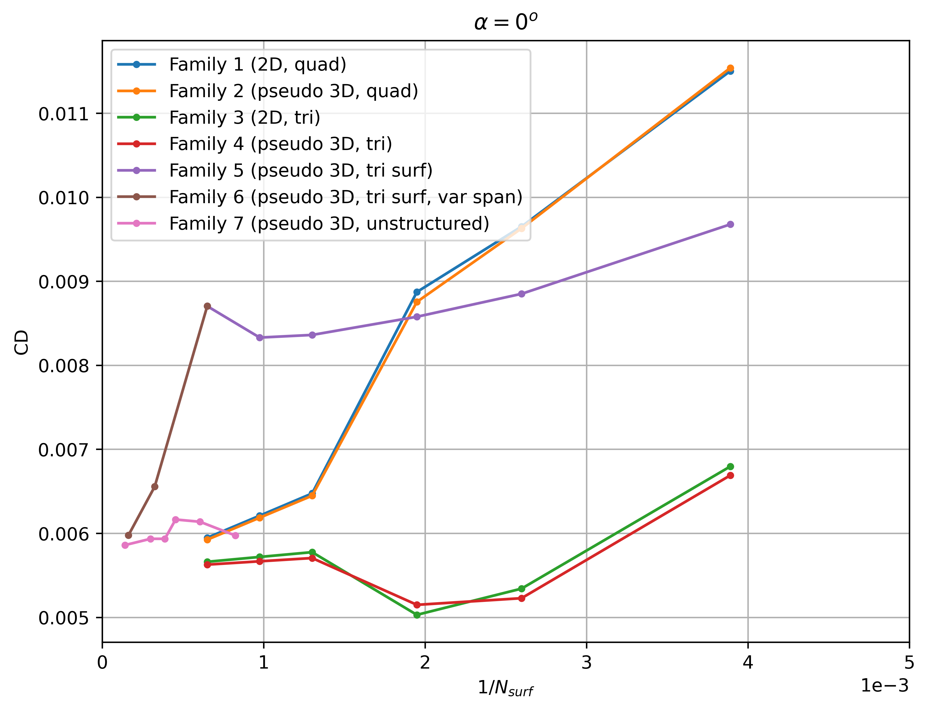
Fig. 6.4.12 Convergence of the drag coefficient with mesh refinement at \(\alpha = 0^o\) for 7 different grid families.

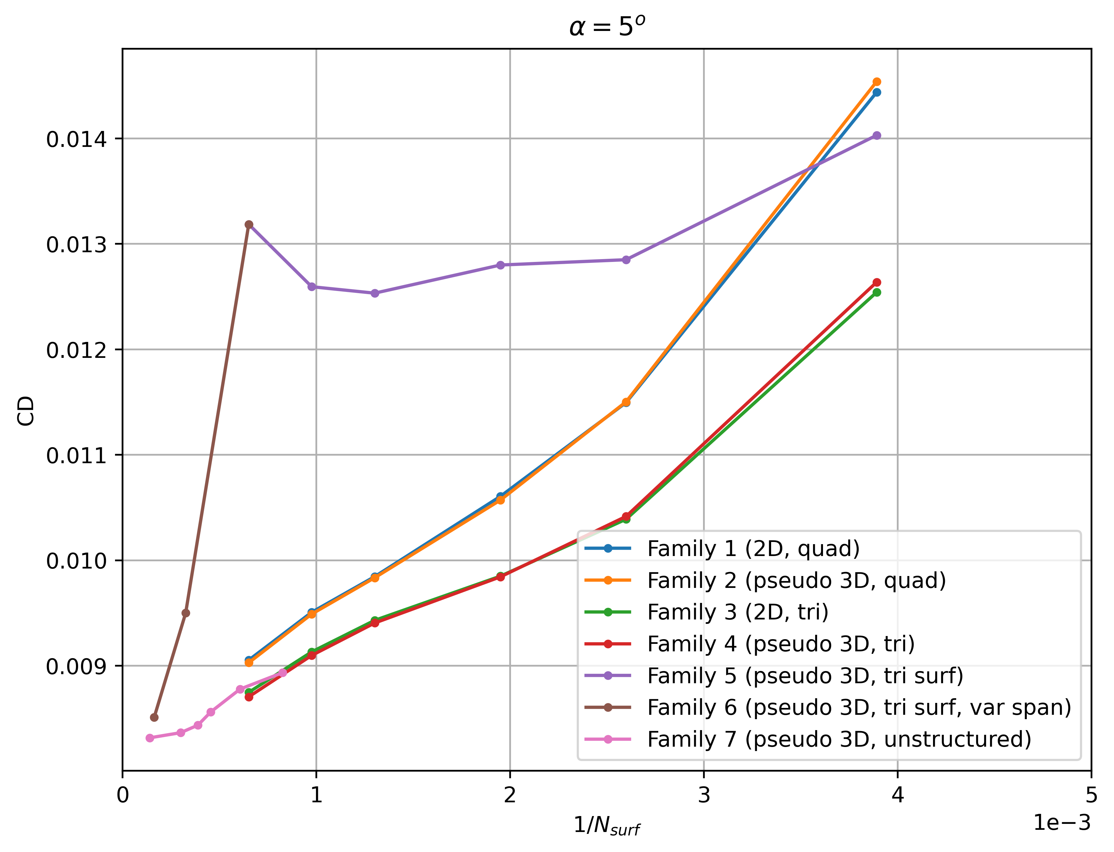
Fig. 6.4.13 Convergence of the drag coefficient with mesh refinement at \(\alpha = 5^o\) for 7 different grid families.

The lift and drag convergence curves indicate a certain degree of non-linearity with mesh refinement for a number of grid families. Families 1-4 appear to converge towards a single value for both lift and drag at both angles of attack for the finest grid levels, however, even finer grids than presented here are required for convergence of the integrated loads. At first glance, the effect of 2D vs pseudo-3D is minimal with the tri meshes showing a lower grid sensitivity (especially from level 2 onwards). Family 5 shows significantly different convergence curves when compared to the other grid families with a high lift and drag prediction and low sensitivity with mesh refinement. Family 6 indicates at first glance that adding nodes in the spanwise direction to the Family 5 grids, aligns the integrated loads with the other grid families. The automated meshing unstructured grids show a lower variation with mesh refinement, although the node counts for these grids is higher than for other mesh families. The reasons for these effects are examined in more detail in the following figures. Firstly, however, the grid convergence of each mesh family is assessed by extracting the skin friction distributions across different grid levels shown in Fig. 6.4.14-Fig. 6.4.17.

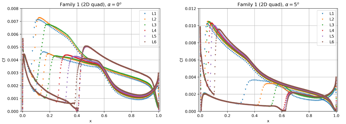
Fig. 6.4.14 Convergence of the skin friction distribution with mesh refinement at two angles of attack for grid Family 1.

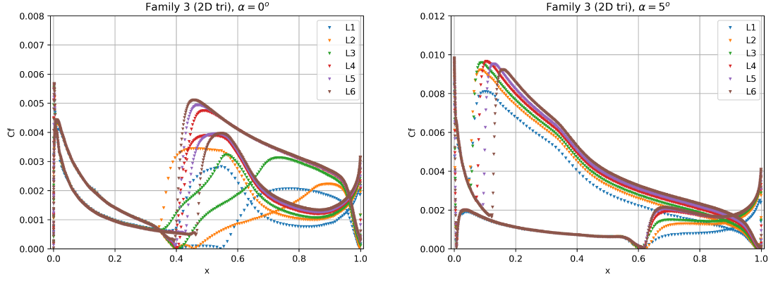
Fig. 6.4.15 Convergence of the skin friction distribution with mesh refinement at two angles of attack for grid Family 3.

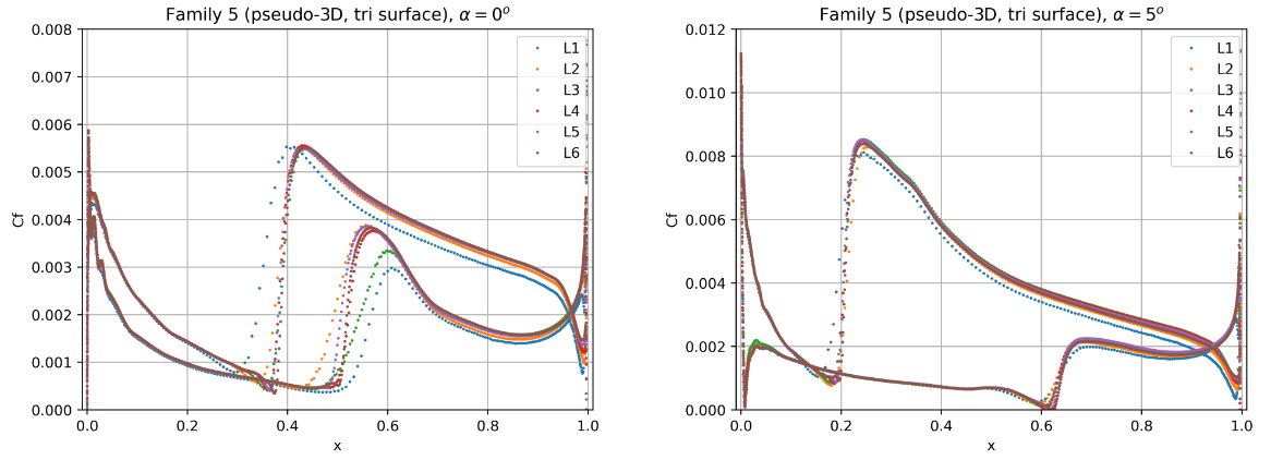
Fig. 6.4.16 Convergence of the skin friction distribution with mesh refinement at two angles of attack for grid Family 5.

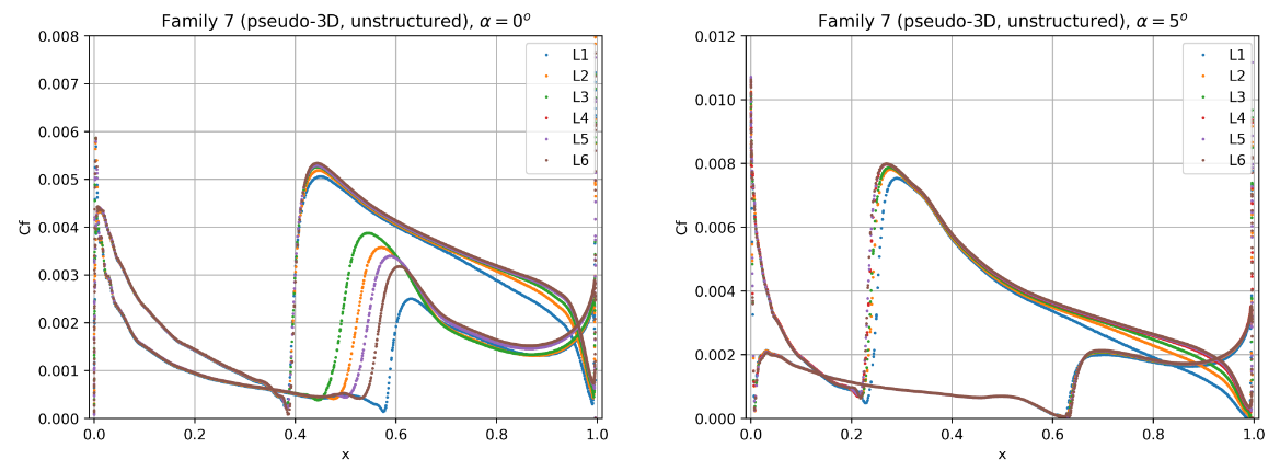
Fig. 6.4.17 Convergence of the skin friction distribution with mesh refinement at two angles of attack for grid Family 7.

The skin friction distributions for grid Family 1 show signs of inadequate grid convergence as the transition locations are still sensitive to mesh resolution. At both angles of attack the transition locations shift aft with mesh refinement. The upper surface at an angle of attack of 0 degrees and lower surface at 5 degrees, show signs of mesh convergence. The transition locations on the lower surface at 0 degrees and upper surface at 5 degrees, continue to move aft showing the requirement for even finer meshes. Grid Family 3 shows similar mesh convergence compared to grid Family 1 for the finest grids (L4-L6). At an angle of attack of 0 degrees, the transition is poorly resolved for mesh levels 1 to 3. At the higher angle of attack, the upper surface shows signs of inadequate mesh convergence. Families 2 and 4 showed similar behaviour to Families 1 and 3 respectively, hence are not shown here. Grid Family 5 shows good signs of mesh convergence, however, the results are analysed further in the section on the sensitivity of the number of spanwise elements. The unstructured meshes which were generated with the automated meshing workflow show much better grid convergence properties than the other grids. The only region that would benefit from further mesh refinement is the lower surface transition prediction for the case at 0 degrees alpha.

6.4.3.3. 2D vs Pseudo-3D

Next 2D versus pseudo-3D predictions are analysed in greater detail. The skin friction distributions are compared between Family 1 and Family 2 as well as Family 3 and Family 4 at two mesh levels, shown in Fig. 6.4.18.

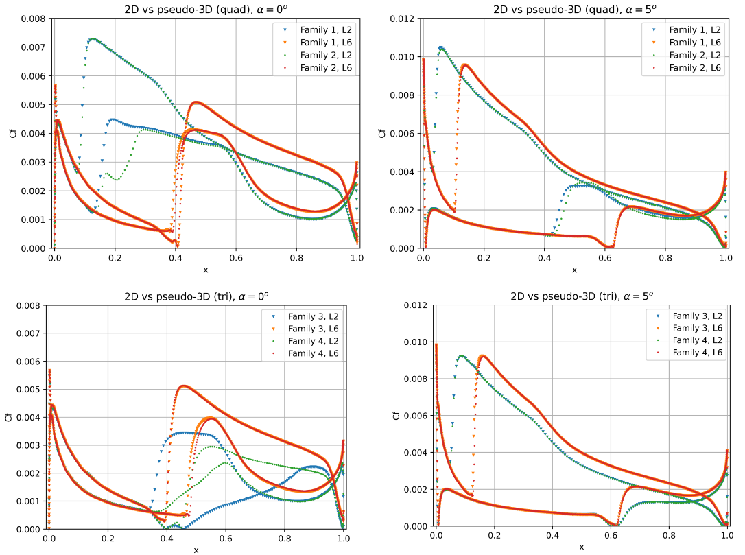
Fig. 6.4.18 Comparison of the skin friction distribution for L2 and L6 grids at two angles of attack for 2D and pseudo-3D grids.

The skin friction distributions show that if the transition is underesolved as is the case for the L2 meshes, some impact of 2D vs pseudo-3D may be observed. However, once the skin friction gradient is resolved well by the mesh, the differences between 2D and pseudo-3D solutions become negligible. A minor sensitivity is seen on the lower surface at an angle of attack of 0, however, as will be seen in the analyses below, the transition location is very sensitive at this condition to the mesh.

6.4.3.4. Spanwise Grid Effects

The effect of number of spanwise elements is also analysed for meshes that contain both quad-type and tri-type elements on the surface. The primary reason for this investigation is that the integrated loads for grid Family 5 were an outlier compared to other grid families. As mentioned previously, an additional quad grid was generated with 40 spanwise nodes that does not belong to any grid family. To examine the effect of number of spanwise nodes, we first look at the surface skin friction and pressure distributions shown in Fig. 6.4.19.

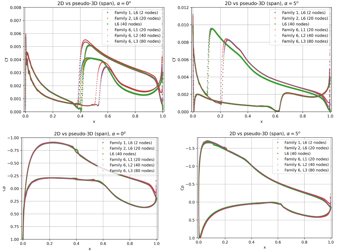
Fig. 6.4.19 Comparison of the skin friction and surface pressure distributions for L6 grids with varying number of spanwise nodes at two angles of attack.

For the quad grids, including Family 1, Family 2 and the grid with 40 nodes, very little sensitivity is seen in both the skin friction and surface pressure distributions, as the curves are pretty much on top of each other. A very minor sensitivity can be seen on the lower surface at 0 degrees angle of attack. The Family 6 grids show a very large sensitivity in the integrated loads, however, the skin friction distributions do not indicate such sensitivity. At both angles of attack the transition locations move slightly aft with mesh refinement, but not enough to cause larger differences in the integrated loads. Looking at the surface pressure distributions however, it can be seen that the tri grids with a low number of spanwise nodes, predict a larger acceleration over the leading edge of the airfoil as indicated by the larger suction peak. The trailing edge pressure recovery is also weaker. Based on these observations, it can be stated that the effect of number of spanwise nodes does not directly impact the transition location, but affects other critical regions of the flowfield to a greater degree. It must, however, be reiterated that the Family 6 grids with a lower number of spanwise nodes are of poorer grid quality due to the high aspect ratio’s of the tet cells. Reducing the decay factor in the volume grid, does not change these observations either. To examine in further detail, exactly what impact the surface grid topology has on the transition location and three-dimensionality of the skin friction distribution, the skin friction contours are extracted at two angles of attack, shown in Fig. 6.4.20-Fig. 6.4.23

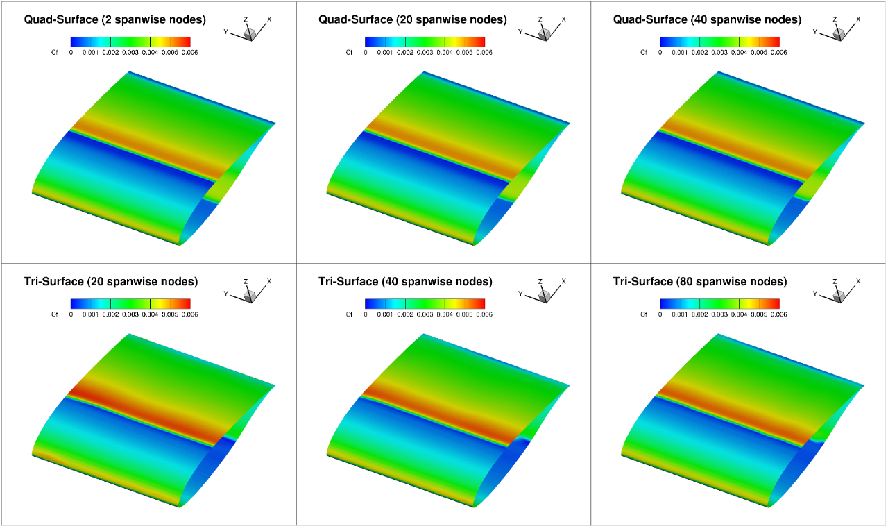
Fig. 6.4.20 Comparison of the skin friction contours on the top surface for L6 grids with varying number of spanwise nodes at 0 degrees alpha.

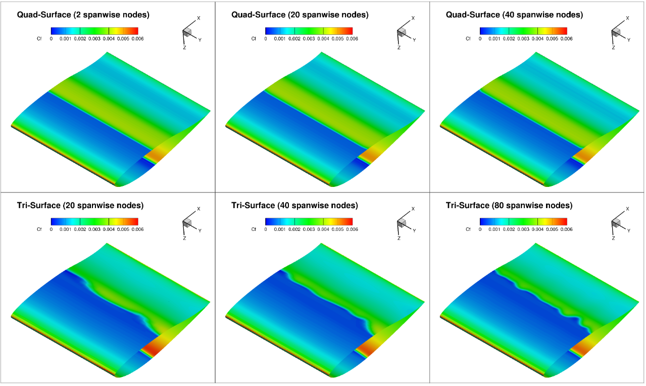
Fig. 6.4.21 Comparison of the skin friction contours on the lower surface for L6 grids with varying number of spanwise nodes at 0 degrees alpha.

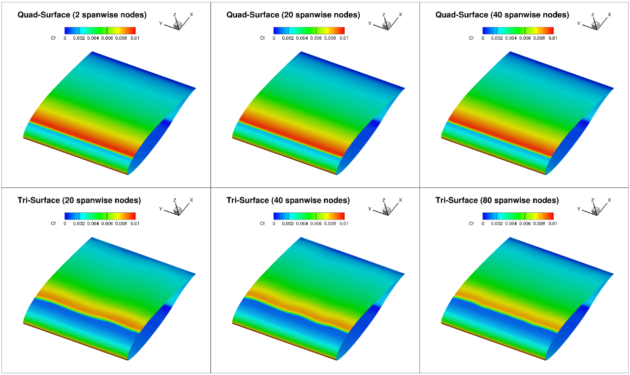
Fig. 6.4.22 Comparison of the skin friction contours on the top surface for L6 grids with varying number of spanwise nodes at 5 degrees alpha.

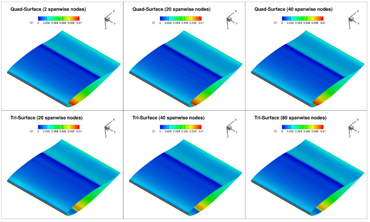
Fig. 6.4.23 Comparison of the skin friction contours on the lower surface for L6 grids with varying number of spanwise nodes at 5 degrees alpha.

The skin friction contours indicate that close to no three-dimensional features are seen in the quad grids. The tri surface grids, however, present a certain degree of three-dimensionality especially in the regions where the transition location was sensitive to grid refinement: the lower surface at 0 degrees angle of attack and the upper surface at 5 degrees angle of attack. At 0 degrees angle of attack, the level of three-dimensionality is fairly significant and irregular, whereas at 5 degrees angle of attack a minor waviness can be seen in the transition location which increases in frequency as the grid is refined.

6.4.3.5. Grid Topology Effects

Analysing the effect of different grid elements further, the skin friction distributions are compared for the level 6 grids across different families Fig. 6.4.24.

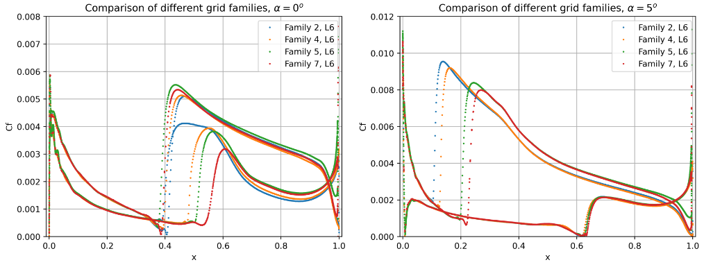
Fig. 6.4.24 Comparison of the skin friction distribution for L6 grids with different element types at two angles of attack.

Based on the skin friction distributions, it is confirmed that the regions of highest grid sensitivity in terms of transition location predictions are the lower surface at 0 degrees angle of attack and the upper surface at 5 degrees angle of attack. Even though fairly fine grids are used here, the transition location varies by over 0.1 chords at these conditions. This correlation, however, is likely to be improved if even finer grids were to be used. The differences are also due to the fact that quad and tri based meshes do not typically show the same integrated loads convergence with mesh refinement even for fully-turbulent solutions. The skin friction contours are extracted for grid Family 7 to assess what levels of three dimensionality is present at the transition locations, presented in Fig. 6.4.25.

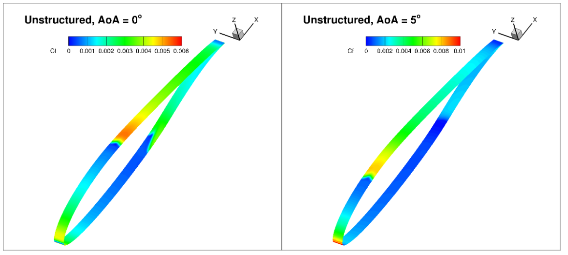
Fig. 6.4.25 Visualization of the skin friction contours for the L6 grids of Family 7 at two angles of attack.

The unstructured grids, also show a certain level of three-dimensionality in the skin friction contours, even though the span was reduced to 0.04 chords. Here, the largest effect can be seen on the lower surface at zero degrees angle of attack.

6.4.3.6. 3D Effects

To examine whether the pseudo-3D results have similar behaviour as a real-life flow scenario, the transition location predictions are compared with a full 3D wing geometry. The 3D simulations were trimmed to the same lift coefficient. A particular focus is put on the level of three-dimensionality of the transition front, for a straight untapered untwisted wing. Firstly, we compare the skin friction coefficient distributions extract at mid-span for the 3D solution, presented in Fig. 6.4.26.

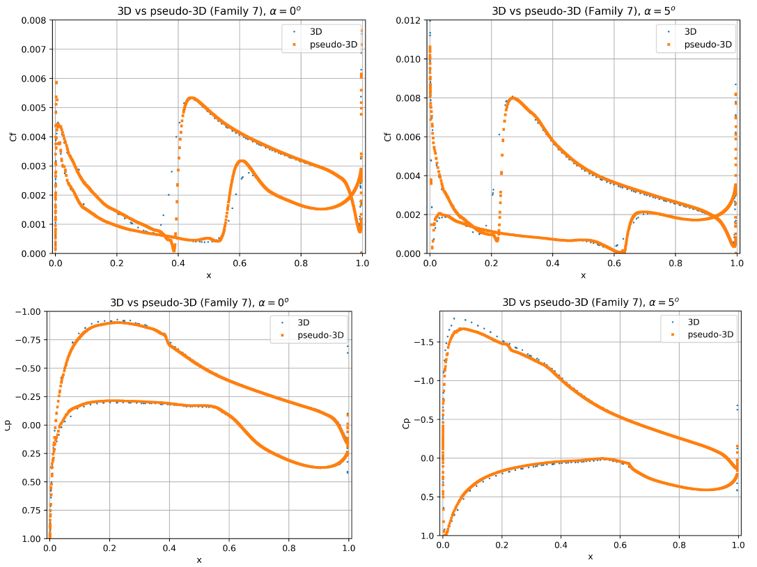
Fig. 6.4.26 Comparison of the skin friction and surface pressure coefficient distribution between pseudo-3D and 3D solutions at two angles of attack.

The 3D geometry results show a high degree of consistency compared to the pseudo-3D unstructured grid results. Some minor differences can be seen especially in the resolution of the skin friction curve gradients for the 3D geometry. This is primarily due to the fact that a L6 grid resolution for a high-aspect ratio wing would lead to very large mesh sizes, hence a coarser mesh is used here. The transition locations are well captured and show good agreement. The surface pressure predictions, however, indicate a higher suction peak at both angles of attack for the 3D geometry. This means that the sectional lift coefficient is higher for the 3D geometry at the mid-span compared to the pseudo-3D case. The 3D sectional lift coefficient varies with span due to the presence of the trailed tip vortices, which is the cause for this difference. Examining the results in further detail, the skin friction distributions are extracted for the 3D wing, shown in Fig. 6.4.27-Fig. 6.4.28.

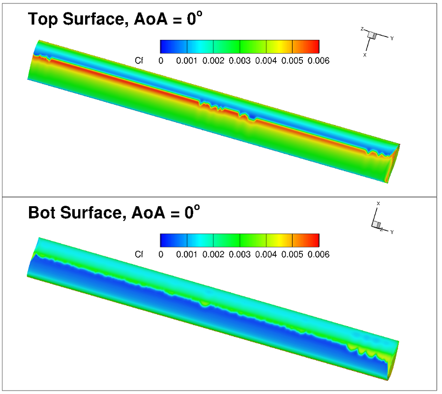
Fig. 6.4.27 Visualization of the skin friction contours for the 3D grids at 0 degrees alpha.

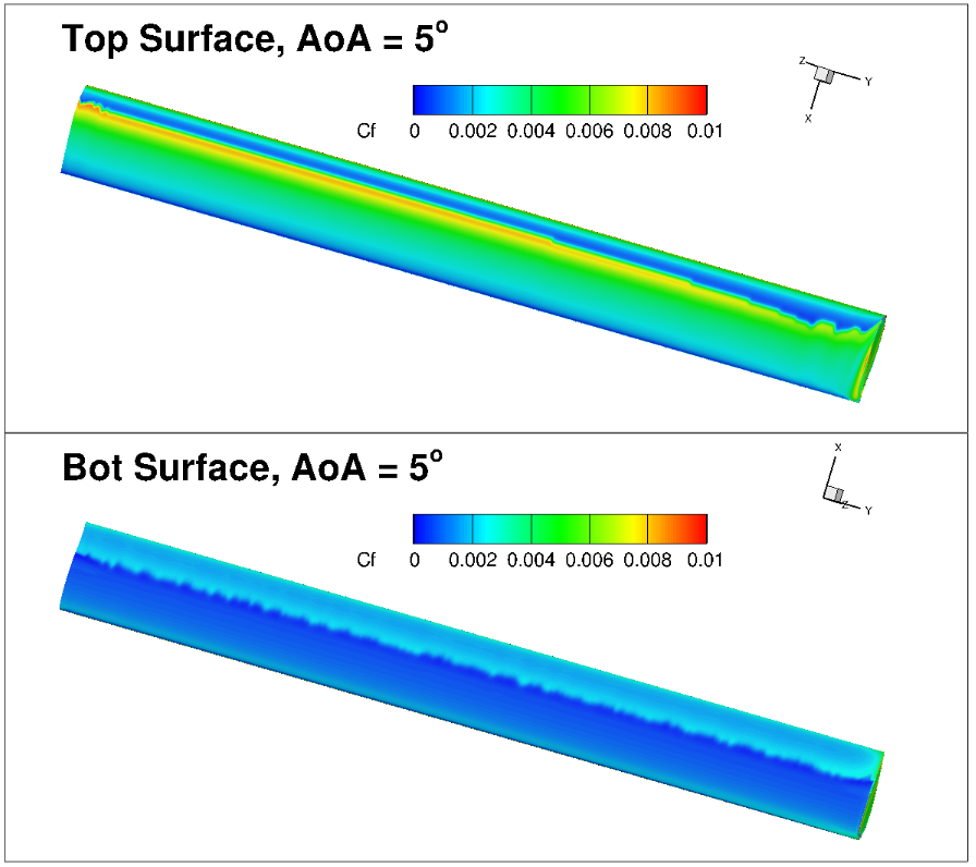
Fig. 6.4.28 Visualization of the skin friction contours for the 3D grids at 5 degrees alpha.

The skin friction distributions show limited three-dimensional effects. At 0 degrees angle of attack some minor irregularity can be seen in the mid-span region of the wing. However, at this condition, the pressure gradients are not significant, hence numerical and discretization sensitivities are emphasized. The 5 degree angle of attack case shows a much more regular transition front. The magnitude of the skin friction peak reduces towards the tip of the wing at both angles of attack. This leads to a spanwise variation in the transition location at 5 degrees angle of attack. Based on the 3D vs pseudo-3D results, it can be stated that the transition locations have good correlation, however, to examine the exact structure of the transition front in terms of three-dimensional effects, finer grids are required.

6.4.3.7. Comparisons with FUN3D/OVERFLOW and Experimental Data

Next we move onto comparisons of the transition predictions using the Flow360 solver with other CFD codes and experimental data. Firstly we compare the integrated loads convergence with mesh refinement with data from OVERFLOW using the SA-AFT transition model and OVERFLOW/FUN3D using the \(\gamma- Re_\theta\) transition model. The mesh convergence study comparisons are presented in Fig. 6.4.29-Fig. 6.4.32.

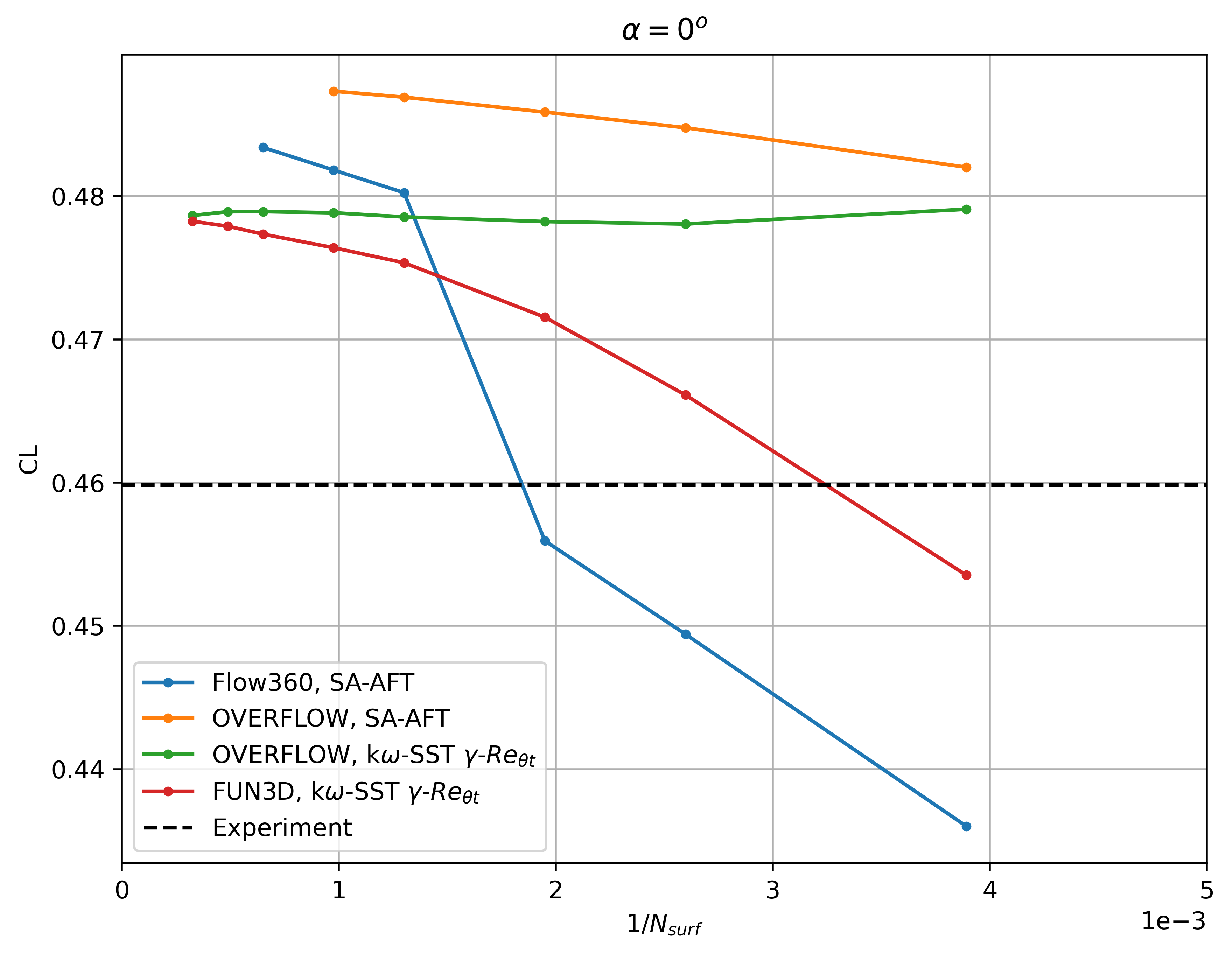
Fig. 6.4.29 Convergence of the lift coefficient with mesh refinement at \(\alpha = 0^o\) for different CFD codes and transition models.

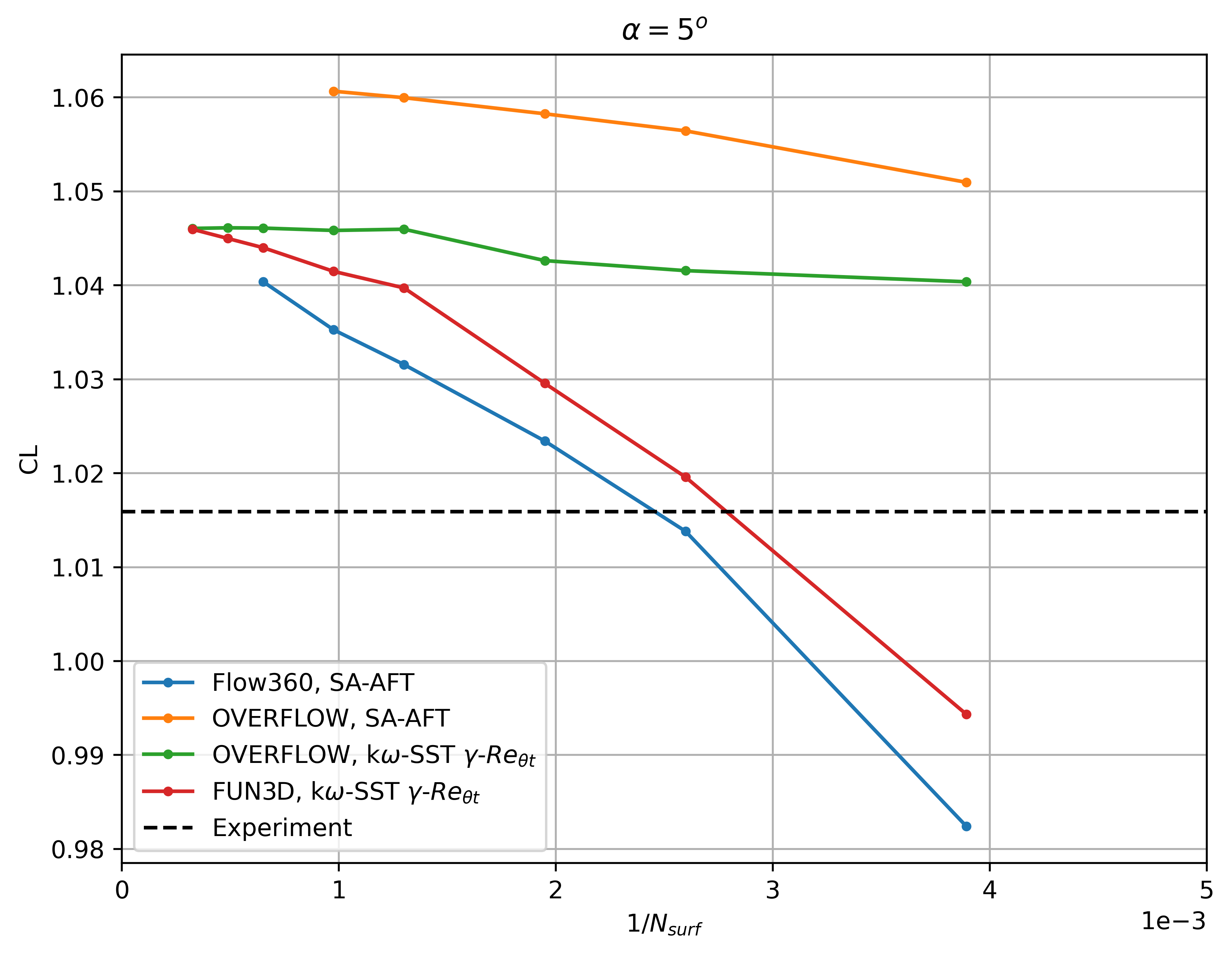
Fig. 6.4.30 Convergence of the lift coefficient with mesh refinement at \(\alpha = 5^o\) for different CFD codes and transition models.

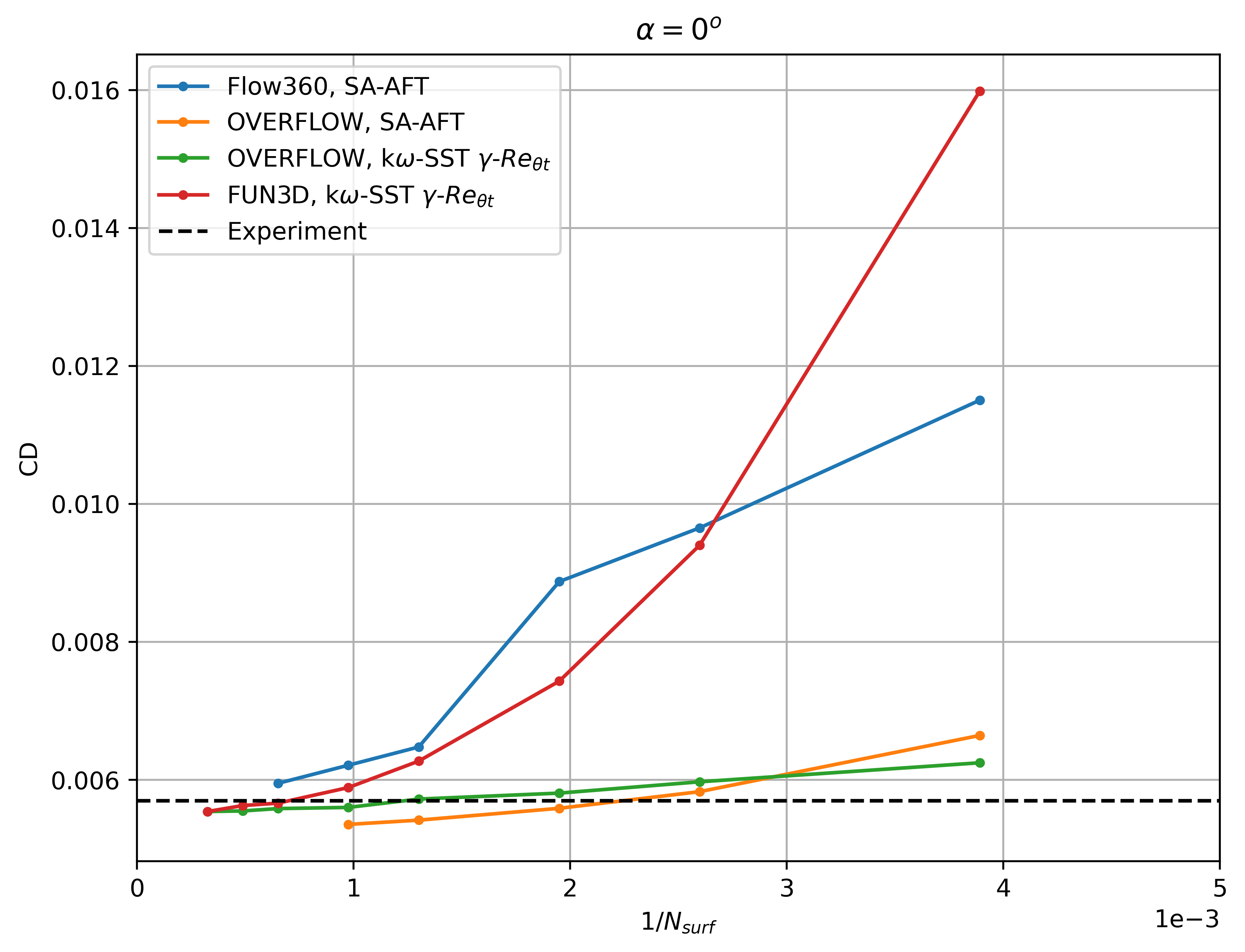
Fig. 6.4.31 Convergence of the drag coefficient with mesh refinement at \(\alpha = 0^o\) for different CFD codes and transition models.

Fig. 6.4.32 Convergence of the drag coefficient with mesh refinement at \(\alpha = 5^o\) for different CFD codes and transition models.

The Flow360 results show similar convergence histories with mesh refinement as FUN3D and OVERFLOW. At 0 degrees angle of attack, a nonlinearity is present going from the L3 to the L4 grid, due to a shift in the transition location on the upper surface. The lift and drag coefficient predictions trend to the same values as other CFD codes, although finer meshes are required to attain mesh convergence, similarly as examined in the \(\gamma- Re_\theta\) results. Differences can also be seen in the values obtained by the two different transition models. The slopes of the intergrated loads convergence curves with mesh refinement, indicate that OVERFLOW is less sensitive to mesh resolution than Flow360 or FUN3D. This is due to the fact that OVERFLOW is a 3rd order cell-centred structured solver, whereas FUN3D and Flow360 are node centred unstructured 2nd order solvers. This means that both FUN3D and Flow360 require a finer grid than OVERFLOW to attain similar levels of accuracy. On the other hand, the primary benefit of unstructured solvers is easier control of the mesh refinement regions and more efficient use of mesh adaptation. The use of mesh adaptation was demonstrated for the NLF(1)-0416 airfoil by Venkatachari et al. who obtained similar predictions as OVERFLOW using adapted meshes in FUN3D for a given grid size. Before performing further comparisons with experimental data and other CFD codes, a finer 2D quad-based mesh was generated with 2.168 million nodes. The skin friction and surface pressure distributions are compared between the different CFD solvers and transition models in Fig. 6.4.33. Note that here, the OVERFLOW and FUN3D predictions based on the \(\gamma- Re_\theta\) model are presented for L8 committee grids (unavailable in the public domain), whereas the OVERFLOW SA-AFT results are presented for the L3 committee grid.

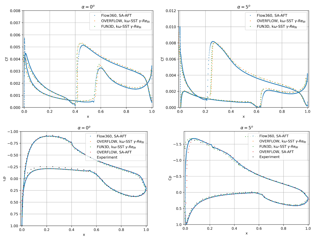
Fig. 6.4.33 Comparison of the skin friction and surface pressure coefficient distribution between different CFD codes and transition models.

The Flow360 skin friction and surface pressure distributions show good agreement with the OVERFLOW and FUN3D solutions. At 0 degrees angle of attack, the transition locations are in excellent agreement with minor deviations in the skin friction coefficient peak values. At 5 degrees angle of attack, the differences are slightly greater, however different transition models and grids were used here. The surface pressure predictions are in good agreement, with similar differences from experimental data observed in all CFD solvers and transition models. Finally, a full alpha sweep is performed and compared with experimental data and the SA-AFT OVERFLOW results (for the L3 committee grid), shown in Fig. 6.4.34-Fig. 6.4.35. Also included are fully-turbulent SA results for both solvers.

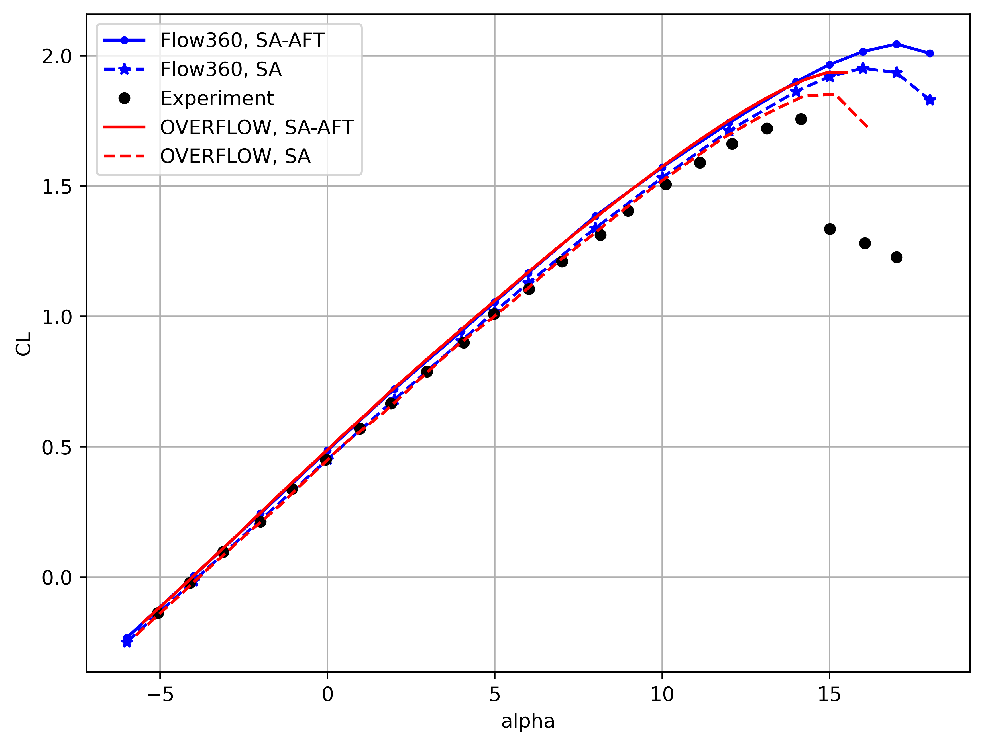
Fig. 6.4.34 Comparison of the CL vs alpha curves between Flow360 and OVERFLOW for the SA and SA-AFT turbulence models.

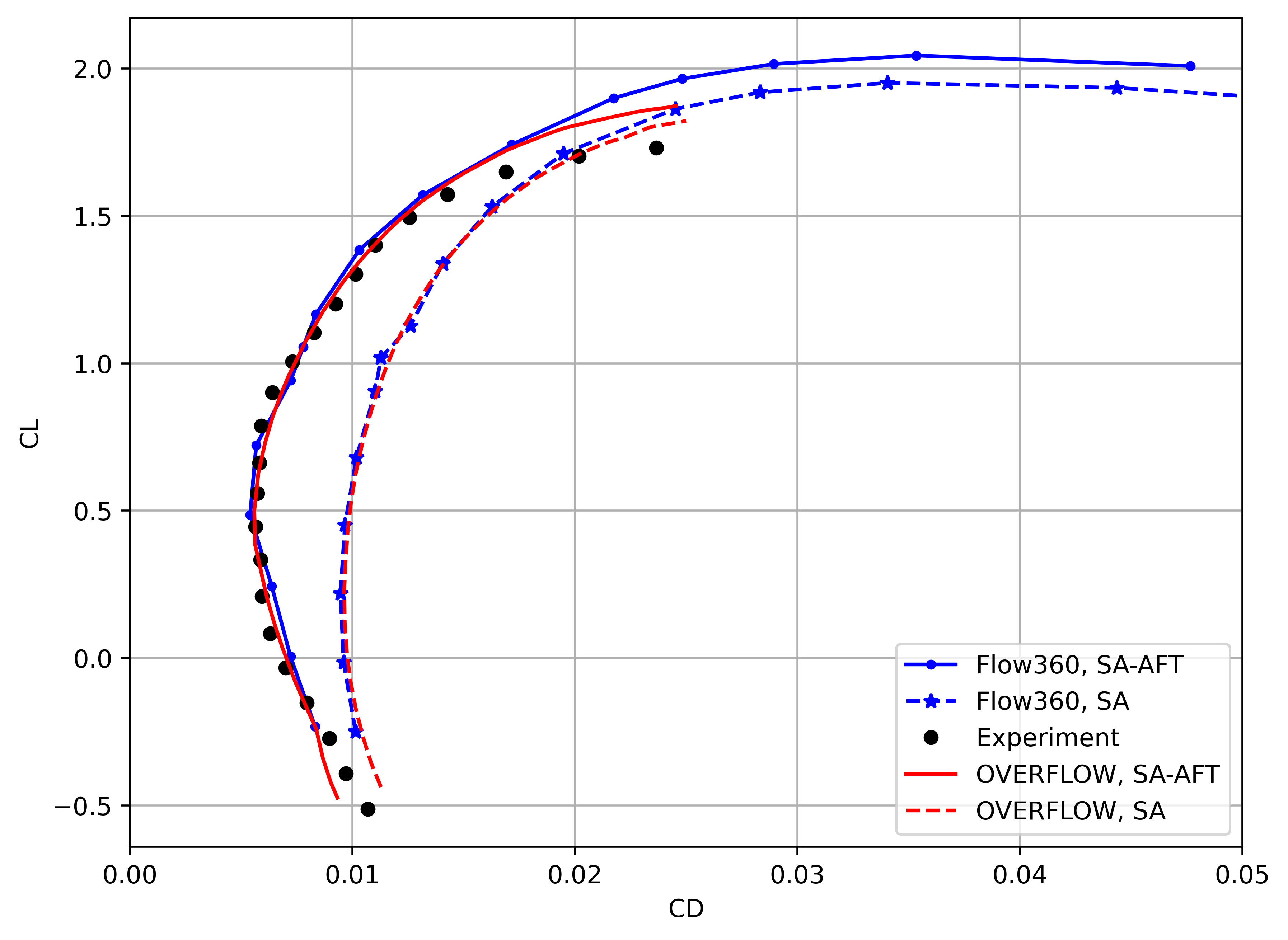
Fig. 6.4.35 Comparison of the drag polar curves between Flow360 and OVERFLOW for the SA and SA-AFT turbulence models.

The alpha sweep results also show good correlation of Flow360 results with OVERFLOW and experimental data. The lift coefficient is slightly overpredicted compared to experiments at a given angle of attack, with excellent agreement with OVERFLOW predictions for both the SA and SA-AFT models. The Flow360 drag polar also shows very good agreement with both experimental data and OVERFLOW results, although the curve is underesolved due to simulations at 2 degree increments in alpha. Both Flow360 and OVERFLOW predict a slightly narrower drag bucket than experiments. The SA-AFT drag polar shows the importance of including transition modeling for the present case, as the drag is overpredicted when using the SA model. Furthermore, DES-based (Detached Eddy Simulation) turbulence modeling is recommended for simulations past stall, as the RANS-based solutions overpredict the lift coefficient at high angles of attack for both Flow360 and OVERFLOW cases.

6.4.4. Conclusions

This case study leads to the following recommendations and conclusions for investigations that include transition modelling:

• Transition location predictions are sensitive to grid resolution. Grid independent results require meshes in the millions of nodes for 2D/pseudo-3D configurations, meaning that for 3D geometries very fine meshes are required. Coarser meshes are able to predict transition with a minor error on the transition location, especially on the airfoil suction side at positive angles of attack and airfoil pressure side at negative angles of attack.

• Quad and Tri based meshes approach the convergence limit from different directions, hence to gain full confidence in the result, a mesh refinement study is always recommended for each configuration.

• Quad-dominant surface meshes with quads oriented in the primary flow direction are preferred to tri-dominant meshes for configurations which can be treated as close to pseudo-3D. The primary reason for this is that tri-dominant surface meshes introduce three-dimensionality due to the discretization even for purely 2D configurations.

• The effect of pseudo-3D vs 2D is negligible for quad-dominant surface meshes. For tri-dominant surface meshes, the effect on the integrated loads is considerable especially when the cell aspect ratio’s are large in the spanwise direction. To minimize the impact of quad vs tri meshes for three-dimensional configurations, the cell aspect ratio’s should be kept below 100 which is the case even for non-transitional calculations. The cell aspect ratio’s are less important for quad-dominant grids.

• Tri-based meshes are generally less sensitive to mesh refinement than quad based meshes although lead to much higher dissipation for coarser meshes in terms of transition location predictions and the gradient resolution of the skin friction curves.

• The Flow360 solver was validated against experimental data and other CFD codes, showing good correlation in the integrated loads and transition location predictions for both the flat plate and NLF(1)-0416 airfoil cases.