6.3. 2D Backward Facing Step

6.3.1. Introduction

The main purpose of this case is validation of the Flow360 solver against experimental data and other CFD solvers, primarily CFL3D. In this study, the simulations are performed using the SA and \(k-\omega\) SSTm turbulence models. The case is part of the NASA Turbulence Modelling Website and has also been evaluated by other CFD solvers such as OVERFLOW in Jespersen et al. The experimental data includes surface pressure, skin friction data, velocity and turbulent shear stress profiles upstream and downstream of the backward facing step in Driver et al. The primary objective of this case is validation for the prediction of reattachment point downstream of the step. Additionally, verification can be performed by comparing with the CFL3D code. Comparisons were also performed using freestream and subsonic inflow boundary conditions.

6.3.2. Simulation setup

A single structured grid with four zones is used, available at the Backward facing step case page of the TMR website. The second finest grid (257x257, 97x257, 385x449, 129x449) is used to perform direct comparisons with CFL3D on the same grid. The grid used in Flow360 was modified for the names and number of boundaries, and is available here. A detailed grid convergence study is not performed here. The grid topology for a coarser level 2 grid is shown in Fig. 6.3.1.

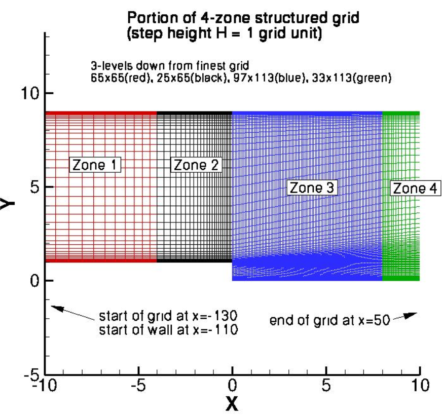
Fig. 6.3.1 Grid topology for the backward facing step study, Level 2 shown (two levels finer grid used in current study).

The flow conditions were set to 36,000 Reynolds number and a Mach number of 0.128. A reference temperature of 298.333K was used. Two different boundary conditions were examined for the inflow boundary conditon. First, a standard freestream boundary condition was used with a specified freestream Mach number. Secondly, a subsonic inflow boundary condition was also used, with a specified pressure and temperature ratio calculated based on isentropic flow relationships (total pressure ratio = 1.011515853 and total temperature ratio = 1.0032768, based on M = 0.128). The outflow boundary condition was set through a static pressure ratio iteratively to ensure that the velocity profile upstream of the backward facing step matched CFL3D data. An outlet static pressure ratio of 1.0108 was used for the freestream inlet boundary condition and 0.99025 for the subsonic inflow boundary condition. Fully-turbulent calculations were performed with the ratio of the freestream value of the SA turbulence field variable (relative to laminar) set to 3, set in Flow360 as a turbulent viscosity ratio of 0.210438. For the k- ω SSTm calculations a turbulent viscosity ratio of 0.009 was used. The case layout is shown in detail in Fig. 6.3.2, whereas the solver inputs are summarized in Table 6.3.1.

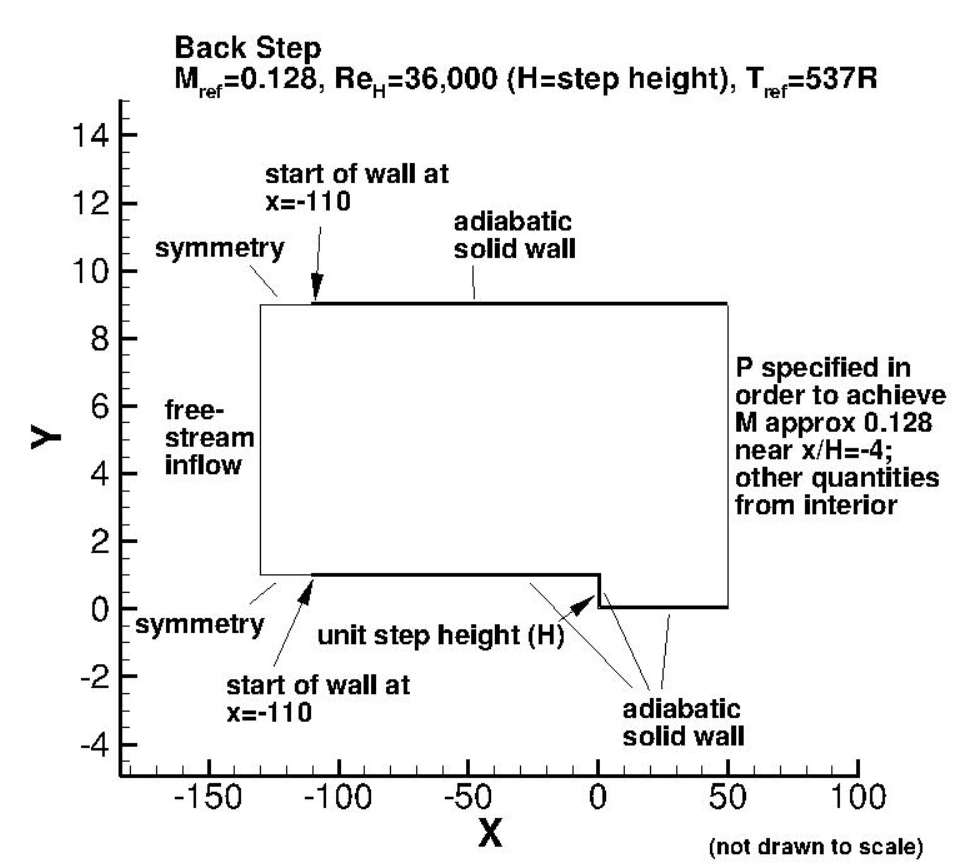
Fig. 6.3.2 Summary of case boundary conditions and conditions for the backward facing step study.

Table 6.3.1 Solver inputs for the backward facing step study.

Parameter	Value
Reynolds number	36,000
Mach number	0.128
Reference temperature	298.333K
Freestream turbulent viscosity ratio	0.210438 (SA), 0.009 (\(k-\omega\) SSTm)
CFL number	100 (reduced to 5)
Inflow total temperature ratio (subsonic inflow b.c.)	1.003277
Inflow total pressure ratio (subsonic inflow b.c.)	1.011516
Outlet static pressure ratio (freestream inflow b.c.)	1.0108
Outlet static pressure ratio (subsonic inflow b.c.)	0.99025

The simulations were performed using a CFL number of 100 ramped up over the initial 2000 iterations. A reduction in CFL to a value of 5 was required at the end of the simulations to ensure convergence to steady state. Contrary to reported results by Jespersen et al and on the TMR website steady-state convergence was obtained when using the k- ω SSTm model, with only a minor oscillation in the final loads. For the majority of cases, a steady residual drop of at least 1e-10 for the flow residuals and 1e-8 for the turbulence residuals was achieved. The Flow360Mesh.json and Flow360.json files are provided for the SA model simulations (compatible with the modified backward facing step grid for number of boundaries and boundary names).

6.3.3. Numerical Results

Firstly, the reattachment locations are compared between Flow360, experimental data and different CFD solvers shown in Table 6.3.2. Note the OVERFLOW code uses the baseline k- ω SST model, whereas the k- ω SSTm model is used by CFL3D and Flow360.

Table 6.3.2 Comparison of reattachment locations between different CFD solvers and experiment for the backward facing step using the SA and k- ω-SSTm turbulence models.

Code	Turb. model	Reattach. loc. (x/H)
Experiment	\(-\)	6.26 \(\pm\) 0.10
CFL3D	SA	6.06
OVERFLOW	SA	6.1
Flow360, Freestream	SA	6.05
Flow360, Subsonic Inflow	SA	6.05
CFL3D	\(k-\omega\) SSTm	6.54
OVERFLOW	\(k-\omega\) SSTm	6.51
Flow360, Freestream	\(k-\omega\) SSTm	6.532
Flow360, Subsonic Inflow	\(k-\omega\) SSTm	6.535

The reattachment location predictions show excellent agreemnt with CFL3D and OVERFLOW predictions. The impact of the inlet boundary condition is not significant, although it must be noted that a different static pressure ratio was used at the outlet, to ensure the boundary layer shape upstream of the step. The SA model predicts earlier reattachement compared to experiment, whereas the k- ω SSTm model predicts a delayed reattachment location.

To verify that correct inflow profile is applied and to verfify the outlet static pressure ratio value, the U velocity and turbulent shear stress profiles are compared upstream of the backward facing step at x/H=-4, shown in Fig. 6.3.3.

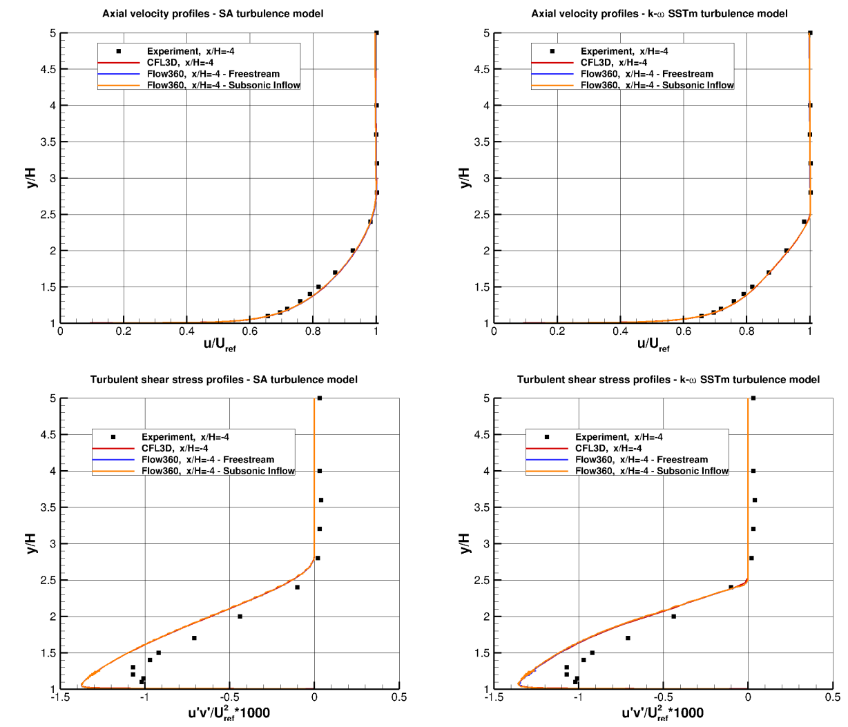
Fig. 6.3.3 Comparison of velocity and turbulent shear stress profiles at x/H=-4 between experimental data, Flow360, and CFL3D for two turbulence models.

Very good agreemnt is obtained for the upstream velocity and turbulent shear stress profiles when comparing Flow360 with CFL3D data. The velocity profile also shows very good agreement with experimental data, with a slight overprediction of the peak turbulent shear stress magnitude. The surface pressure and skin friction coefficients are analysed next, and are compared with the CFL3D code and experimental data in Fig. 6.3.4-Fig. 6.3.7. The surface pressure curves were translated to ensure a surface pressure coefficient of zero at x/H=40, as suggested on the TMR backward step case study page.

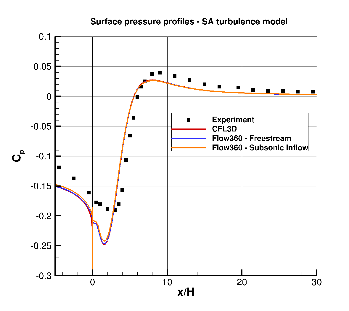
Fig. 6.3.4 Comparison of the surface pressure coefficient data between Flow360, CFL3D and Experiment for the SA turbulence model.

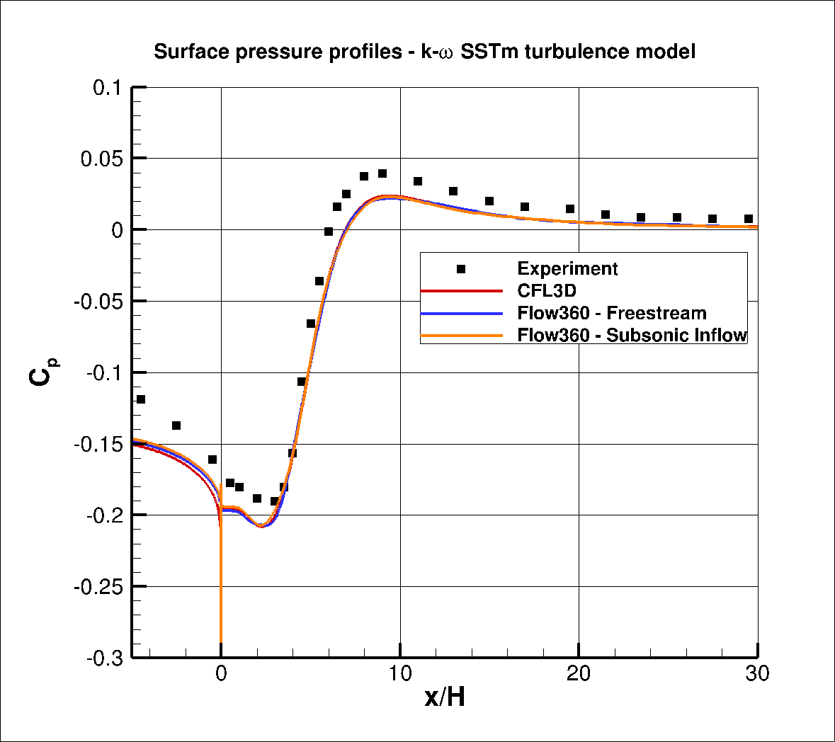
Fig. 6.3.5 Comparison of the surface pressure coefficient data between Flow360, CFL3D and Experiment for the k- ω SSTm turublence model.

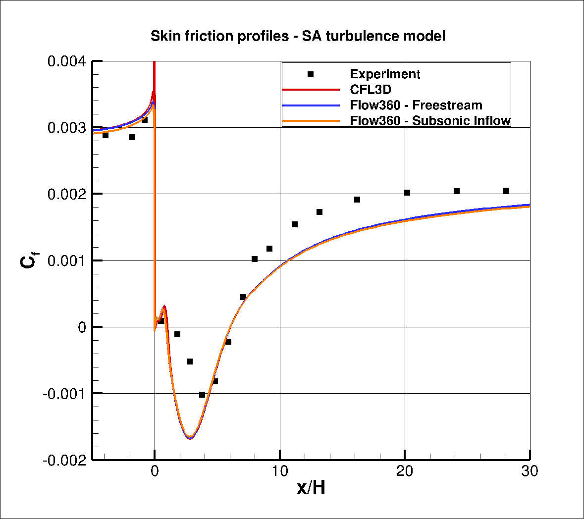
Fig. 6.3.6 Comparison of the surface skin friction coefficient data between Flow360, CFL3D and Experiment for the SA turbulence model.

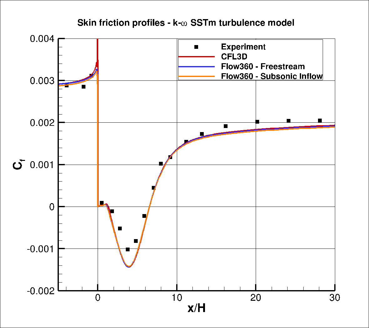
Fig. 6.3.7 Comparison of the surface skin friction coefficient data between Flow360, CFL3D and Experiment for the k- ω SSTm turublence model.

Excellent agreement is obtained between the Flow360 and CFL3D results for both the SA and k- ω SSTm model. The main region where differences can be seen is at x/H = 0.0 where a spike can be seen in the skin friction CFL3D skin friction data not present in the Flow360 results, which in turn exhibit a spike in the surface pressure coeffiicent data. This discontinuity is likely to be due to the high \(y^+\) present on the backward facing step surface. The different inlet boundary condition leads to a slighly lower magnitude of the negative pressure peak and lower skin friction for the subsonic inflow, although these differences are fairly insignificant. Compared to experiments, the use of the k- ω SSTm model improves the skin friction curve slope as the flow reattaches compared to the SA model. For the surface pressure coefficient, the agreement is improved in the region of the separated flow, although better agreement is seen with experment with the SA model after the flow reattaches.

Further analysis is performed by comparing the velocity profiles including the turbulent shear stress at four locations downstream of the backward facing step with data from CFL3D and experiment. The data is normalized by a \(U_{ref}\) for the U and V velocities, and \(U_{ref}^2\) for the turbulent shear stress. The velocity profiles for the two turbulence models are compared in Fig. 6.3.8. The data was extracted using two line probes with uniformly spaced points in Tecplot (one finer line probe for the inner portion of the boundary layer and one coarser line probe for the outer portion). This was done, as the gradients were computed in Tecplot and using the direct CFD data leads to discontinuities in the turbulent shear stress profiles.

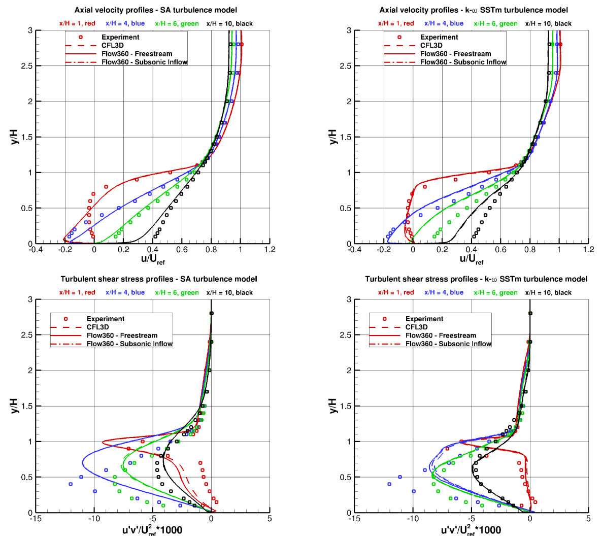
Fig. 6.3.8 Comparison of velocity and turbulent shear stress profiles at four locations downstream of the backward facing step between experimental data, Flow360, and CFL3D for two turbulence models.

The velocity and turbulent shear stress profiles once again indicate that the use of the subsonic inflow boundary condiiton does not have a significant impact although some minor variation can be seen in the turbulent shear stress profile for the k- ω SSTm model at x/H=4. Comparing CFL3D and Flow360 results, the velocity profiles are nearly identical for both turbulence models. A slightly higher turbulent shear stress is seen between y/H=0 and y/H=1 for Flow360 when compared to CFL3D for the SA model, which is likely to be due to the high \(y+\) on the backward facing step wall. For the k- ω SSTm some slight variation can only be seen at x/H=4. Compared to experiment, the SA model predicts better agreement at location x/H=6 and x/H=10 whereas the k- ω SSTm model performs better at x/H=1 and x/H=4, which is seen for both the velocity and turbulent shear stress profiles.

Overall, the results between Flow360, experimental data and other CFD codes show a high degree of consistency leading to further validation and verification of the Flow360 solver. The solver version release-22.2.3.0 was used throughout this study.