5.1. NACA 0012 Low Speed Airfoil#
Introduction#
The purpose of this case study is to verify and validate the functionality of the Flow360 solver and the implementation of the Spalart-Allmaras (SA) and Menter’s \(k - \omega\) shear stress transport (SST) turbulence models, with respect to the NACA 0012 low speed airfoil validation case. This is one of the cases originally provided by the NASA Langley Turbulence Modeling Resource database with accurate and up-to-date information on widely-used turbulence models, as also described by the ONERA-elsA website. Recent high-accuracy numerical investigations on asymptotic grid convergence behaviors over three families of nested grids are described on this NASA-LaRC-TMR webpage. Similar validation results from OVERFLOW were documented by Jespersen et al.
In this study, Reynolds-averaged Navier-Stokes (RANS) simulations utilizing the SA and the SST turbulence models were performed at the same operating conditions as given on those webpages. According to these major conclusions: 1st, the trailing edge streamwise spacing has profound influence on the airfoil lift and moment results, and the grid of Family II yields the most accurate results; 2nd, numerical schemes incorporated with 2nd-order accuracy for turbulence advection are desirable for better asymptotic grid convergence; in the current validation cases, the grid of Family II at Level-4 and 2nd-order accuracy for turbulence model equation were utilized. This grid resolution is comparable to that used in the reference validation cases. Current numerical results were validated with respect to available experimental data, as well as other CFD results where appropriate.
Mesh and Flow Configuration#
From the three series of nested grids with varying trailing edge streamwise spacing, available from this NASA webpage, we used the grid of Family II at Level-4 (FMLY2GL4, with a grid resolution of 897 x 2 x 257) for this validation. The geometry and the mesh of this quasi-3D CFD model are shown in Fig. 5.1.1. As seen, the grid has a C-type topology, wrapping around the airfoil from the downstream farfield, around the lower surface to the upper, then back to the downstream farfield again. Also, in the wake region, the grid connects to itself in a point-matched manner. The chord length is scaled to unity, and the grid unit is taken to be meter. The origin of the grid coordinates is at the leading edge of the airfoil. The x-axis is in alignment with the chord line. Also, the grid is stretched for one spanwise cell in the negative y direction with the grid spacing of one unit length. For this validation case, the original NASA grids are converted from ADF to HDF5 data format and are available here.
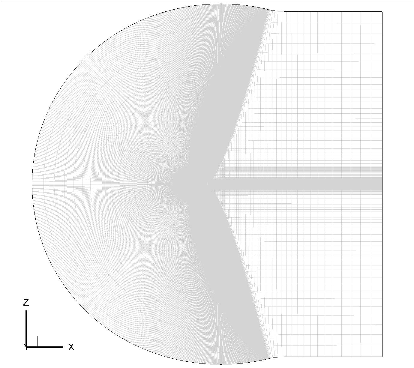
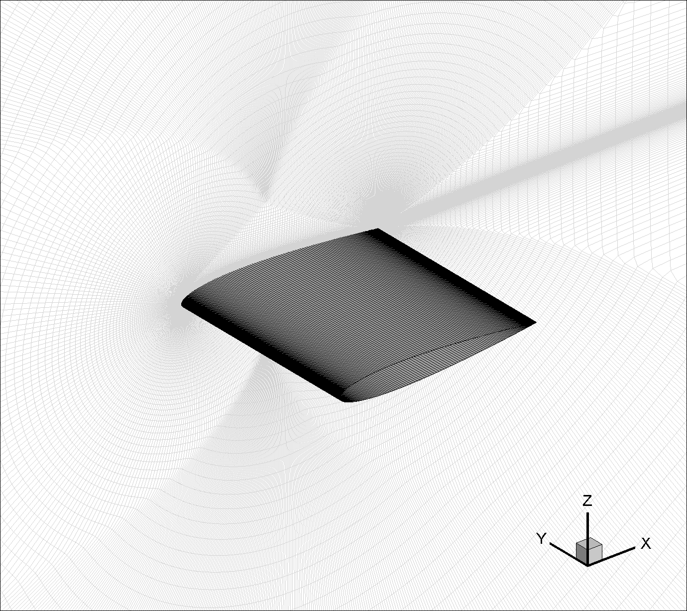
Fig. 5.1.1 Quasi-3D CFD model of NACA 0012 airfoil (Family II, Grid Level-4).#
As suggested by NASA-LaRC-TMR and ONERA-elsA, for this essentially incompressible flow, the freestream Mach number is \(M_{\infty} = 0.15\), the Reynolds number per chord length is \(Re_{c} = 6 \times 10^6\), and the reference temperature is \(T_{ref} = 300 K\). The turbulent flow past the airfoil was simulated at each of three angles of attack, i.e. \(\alpha = 0^o\), \(10^o\) and \(15^o\). Table 5.1.1 summarizes the key flow configuration parameters for Flow360. Detailed descriptions are available for the nondimensional inputs.
Parameters |
Units |
Values |
Notes |
|---|---|---|---|
\(L_{gridUnit}\) |
\(m\) |
\(1\) |
Grid unit length |
\(Re_{L_{gridUnit}}\) |
\(6 \times 10^6\) |
Reynolds number |
|
\(M_{\infty}\) |
\(0.15\) |
Freestream Mach number |
|
\(T_{ref}\) |
\(K\) |
\(300\) |
Reference temperature |
\(\frac{\mu_{t}}{\mu_{\infty}}\) |
Freestream turbulent viscosity ratio |
||
\(0.210438\) |
default for SA model within Flow360 |
||
\(0.009\) |
the default value is \(0.01\) for SST model within Flow360 |
||
\(\alpha\) |
\(deg\) |
\(0, 10, 15\) |
Angle of attack |
\(\text{CFL}\) |
\(100\) |
CFL number |
|
\(\text{AbsTol(NS)}\) |
\(\text{1E-12}\) |
Residual convergence tolerance for NS equations |
|
\(\text{AbsTol(SA/SSTm)}\) |
\(\text{1E-10}\) |
Residual convergence tolerance for SA/SST(m) equations |
|
The “NoSlipWall” boundary condition is applied to the adiabatic viscous surface of the airfoil, and “SlipWall” is used as the symmetry condition in the spanwise direction. The “Freestream” boundary condition is utilized in the farfield, together with the default value of the freestream “turbulentViscosityRatio”, i.e. \(\frac{\mu_t}{\mu_{\infty}} = 0.210438\) for the SA model. This is equivalent to the boundary value based on the SA approximate turbulent kinematic viscosity \(\tilde{\nu}\), i.e. \(\frac{\tilde{\nu}}{\nu_{\infty}} = 3\), as used in the CFL3D predictions. More descriptions about these freestream turbulence boundary conditions can be found from this NASA webpage on the Spalart-Allmaras turbulence model.
Similarly, for the SST model, the value of \(0.009\) is used for the freestream “turbulentViscosityRatio”, i.e. \(\frac{\mu_t}{\mu_{\infty}} = 0.009\). The same value is used in the reference results, such as those CFL3D predictions, where a freestream turbulence intensity, i.e. \(T_u = \frac{u_{rms}}{U_{\infty}} = 0.052\%\) was also specified. More descriptions about these freestream turbulence boundary conditions can be found from this NASA webpage on Menter’s SST turbulence model. Notably, a modified version of the SST turbulence model was incorporated into CFL3D. This is denoted as the SST(m) in Table 5.1.1 and the following. As described on the NASA webpage, this simplified version is exact for incompressible flows and is considered typically a very good approximation, except perhaps for very high Mach numbers. This is also the version implemented in Flow360.
Steady-state solutions were computed iteratively, utilizing 2nd-order schemes for both the time averaged Navier-Stokes and the turbulence model equations. For the former, the CFL number was gradually ramped up to 100. Typically, the values of the absolute nonlinear residual convergence tolerances were set to be \(1 \times 10^{-12}\) and \(1 \times 10^{-10}\) for the RANS and the turbulence model equations, respectively. The definitions of the angle of attack \(\alpha\) and the sideslip angle \(\beta\), with respect to the grid coordinates, are given as EQ_FreestreamBC in the non-dimensional inputs knowledge base.
SA/SA-RC Model Results#
Two-dimensional steady viscous mean flows past the NACA 0012 airfoil were simulated at the aforementioned operating conditions. Aerodynamic characteristics were visualized through contour plots of Mach number and turbulent viscosity ratio on the longitudinal cut-plane at \(y = -0.5\). The results of the RANS simulations based on the SA model with the R/C correction are shown in Fig. 5.1.2, Fig. 5.1.3 and Fig. 5.1.4 for the three angles of attack, respectively.
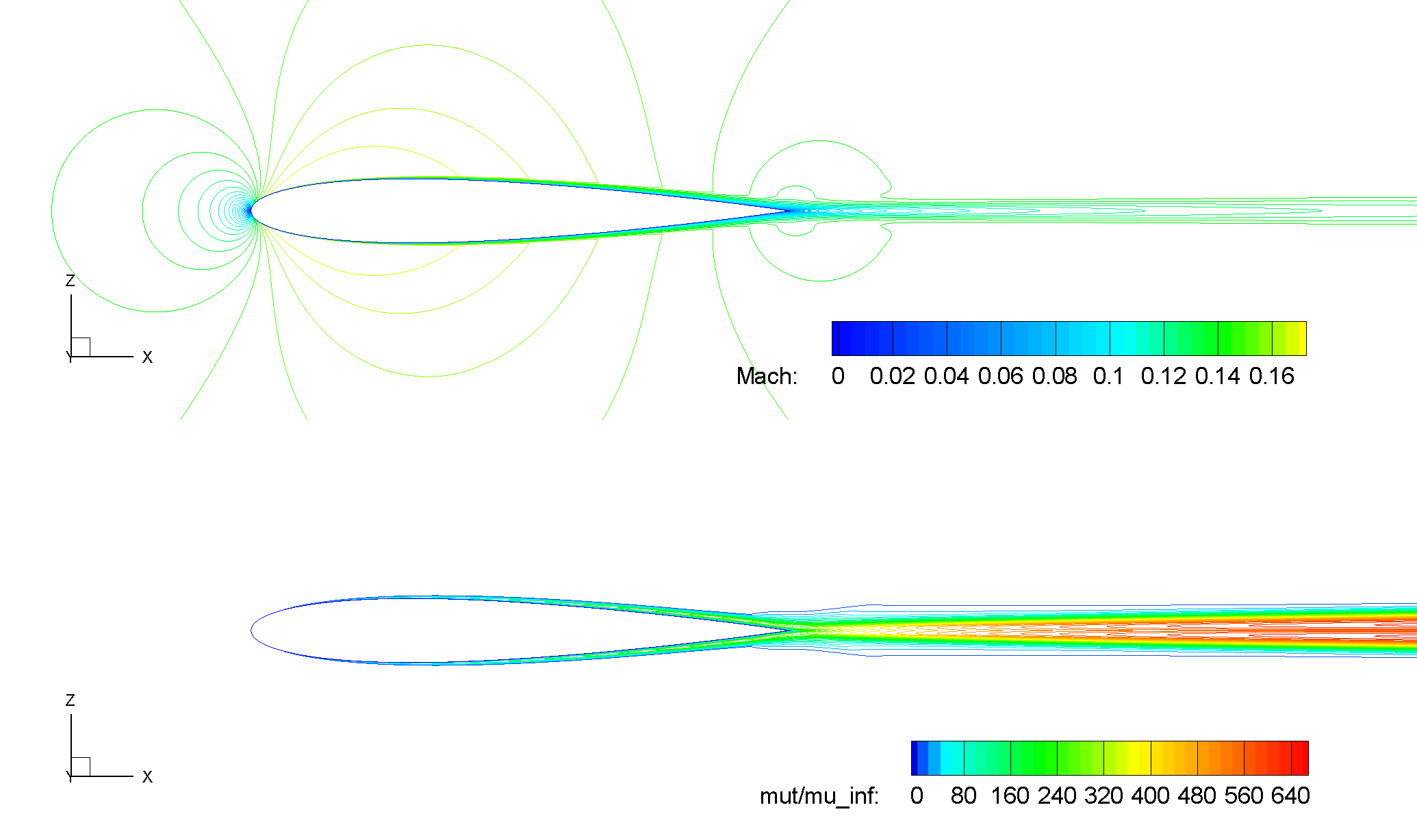
Fig. 5.1.2 Contours of Mach number and turbulent viscosity ratio, NACA 0012, SA-RC, \(\alpha = 0^o\).#
As seen from the above figure, for the zero lift condition at \(\alpha = 0^o\), symmetric flow patterns are established along the chord line at \(z = 0\).
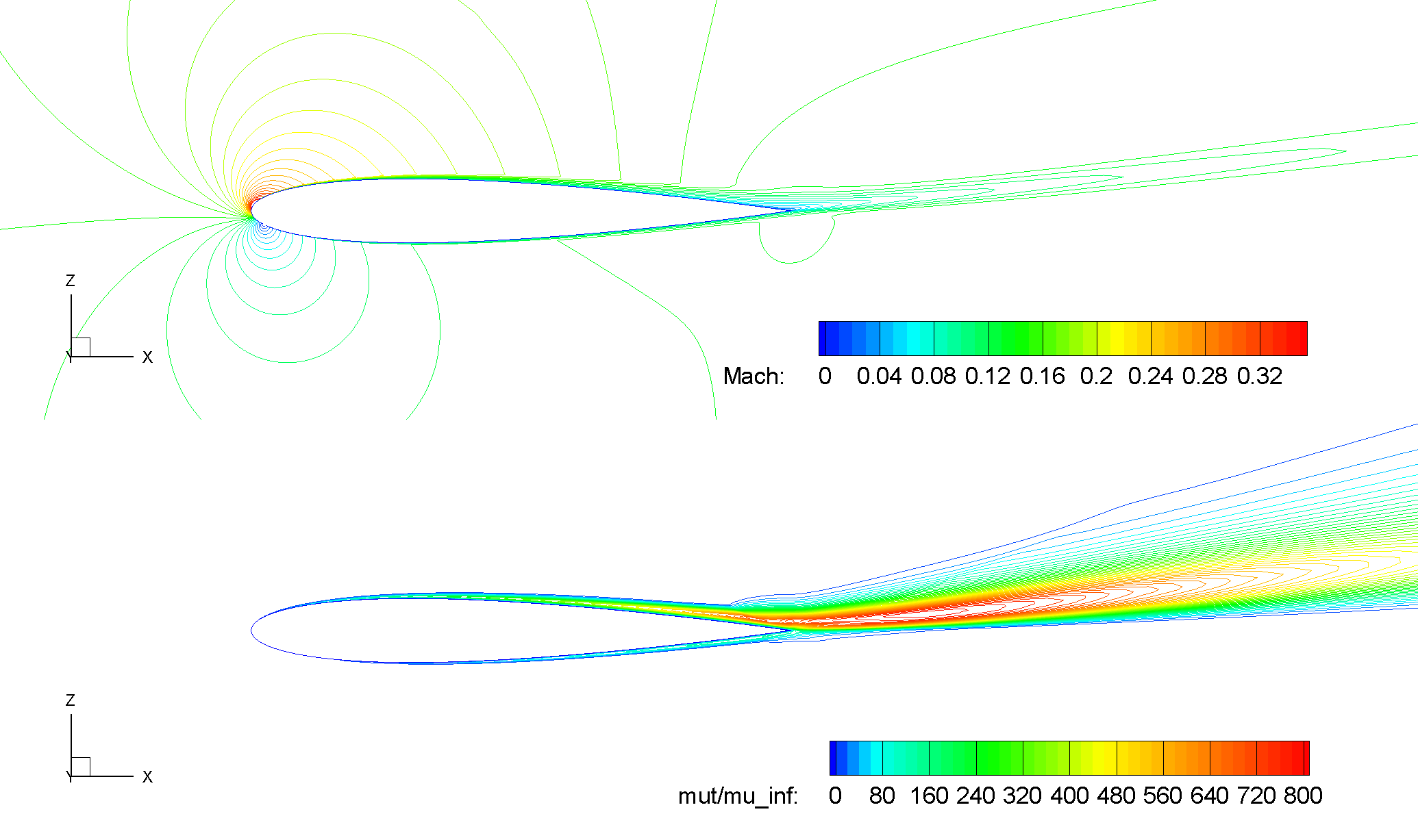
Fig. 5.1.3 Contours of Mach number and turbulent viscosity ratio, NACA 0012, SA-RC, \(\alpha = 10^o\).#
For a relatively high lift condition at \(\alpha = 10^o\), a large wake region trailing down from the airfoil is observed.
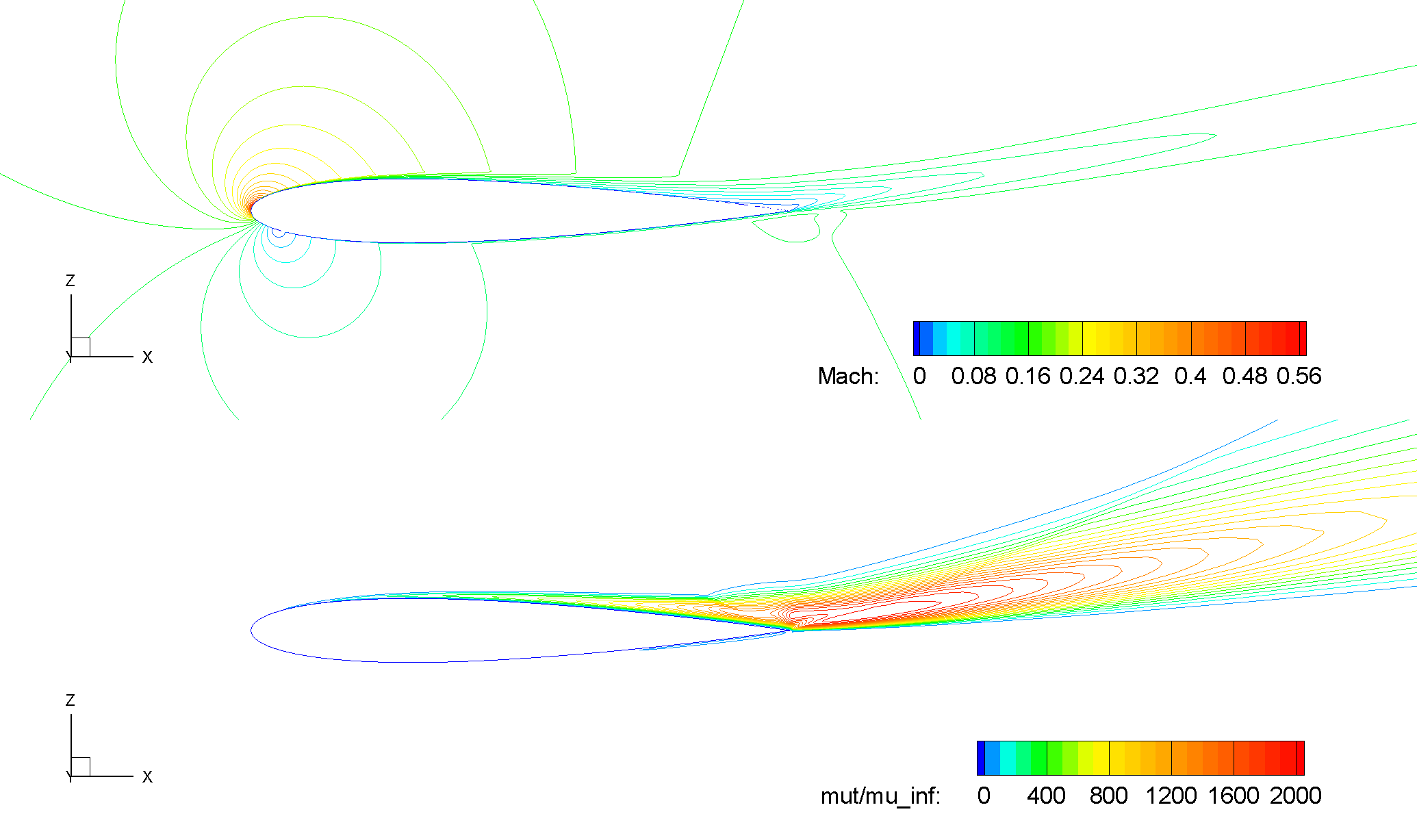
Fig. 5.1.4 Contours of Mach number and turbulent viscosity ratio, NACA 0012, SA-RC, \(\alpha = 15^o\).#
Also, as expected, at a higher angle of attack \(\alpha = 15^o\) towards the operating condition for \(C_{L,max}\), the flow starts to separate from the upper surface near the trailing edge. This is shown in the above figure where detachment of the contour line of \(M = 0\) occurs at a more detailed level.
For these operating conditions, surface distributions of pressure and skin friction coefficients, i.e. \(C_p = \frac{p - p_{\infty}}{0.5 \cdot \rho_{\infty} \cdot U^2_{ref}}\) and \(C_f = \frac{\tau_w}{0.5 \cdot \rho_{\infty} \cdot U^2_{ref}}\), are examined in Fig. 5.1.5, Fig. 5.1.6 and Fig. 5.1.7, with respect to reference data. In these figures, Flow360 results are indicated as the red solid and the green dashed lines for the SA model without and with the R/C correction, respectively. The corresponding CFL3D results are shown as the blue dashed and dash-dot lines. Experimental data are given as symbols. Notably, these measurements of \(C_p\) were made at a lower Reynolds number \(Re_c = 2.88 \times 10^6\) by Gregory and O’Reilly.
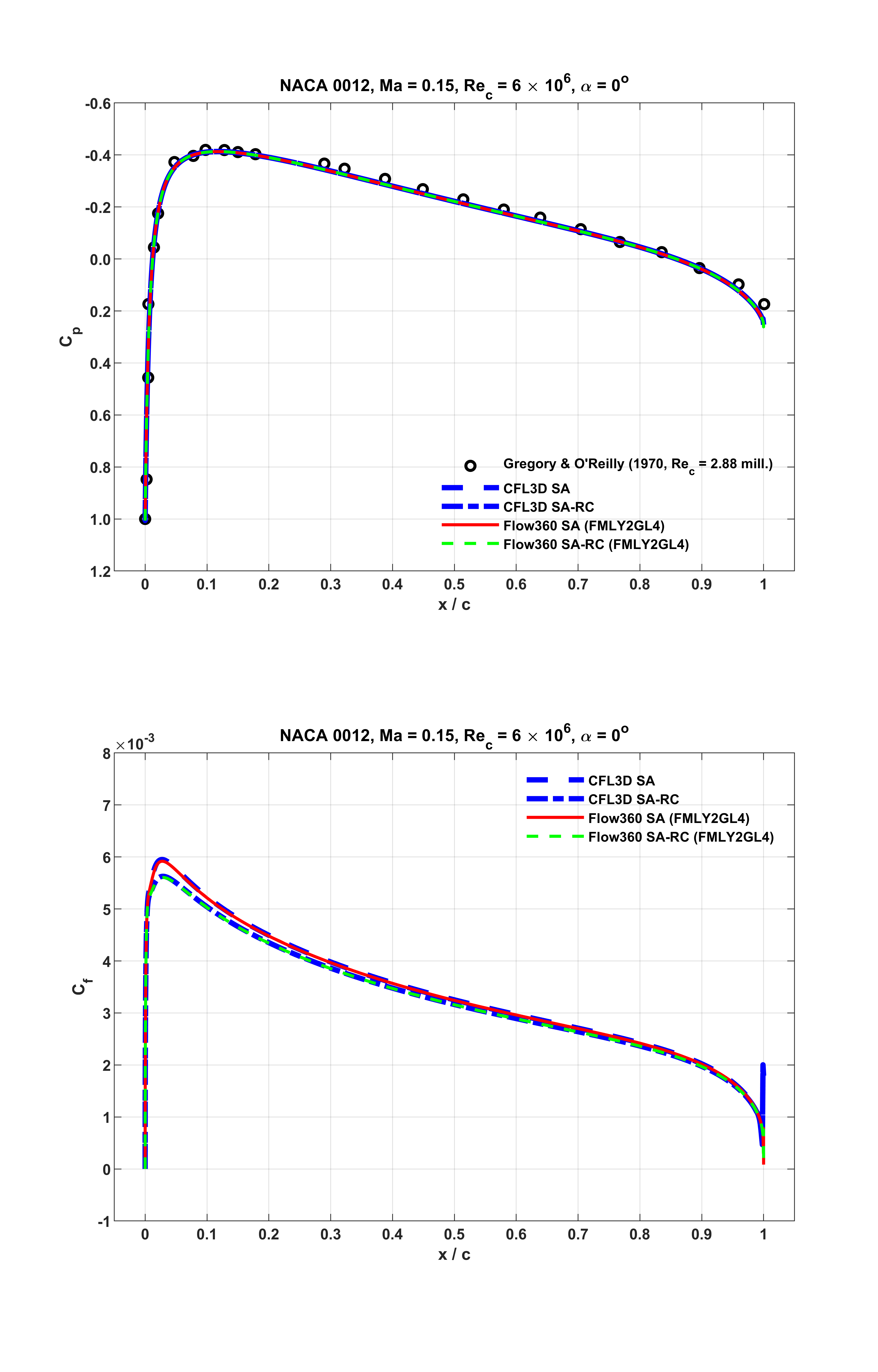
Fig. 5.1.5 Surface distributions of \(C_p\) and \(C_f\), NACA 0012, \(\alpha = 0^o\).#
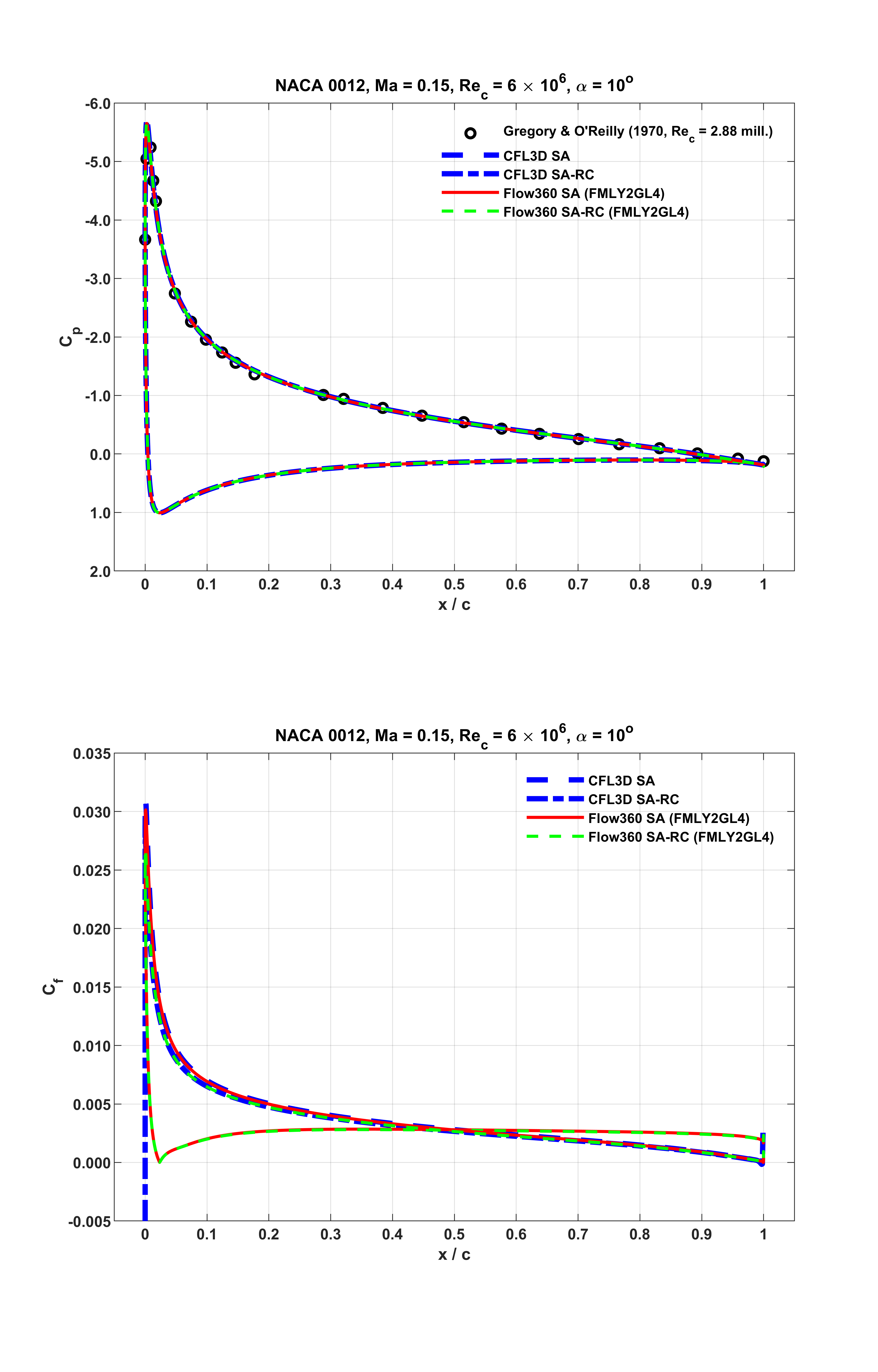
Fig. 5.1.6 Surface distributions of \(C_p\) and \(C_f\), NACA 0012, \(\alpha = 10^o\).#
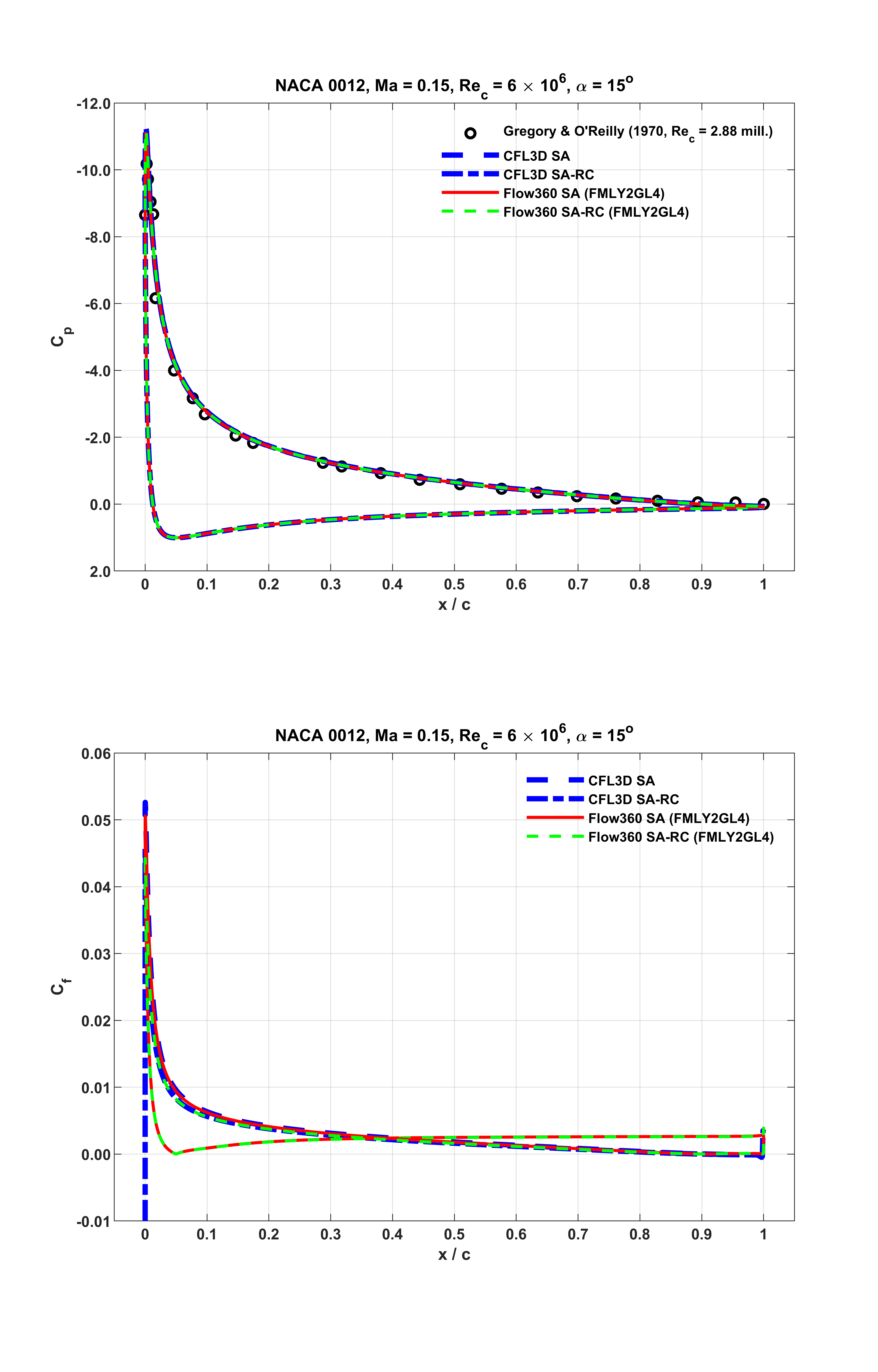
Fig. 5.1.7 Surface distributions of \(C_p\) and \(C_f\), NACA 0012, \(\alpha = 15^o\).#
As seen from the above figures, at all the three distinct lift conditions, Flow360 predictions accurately capture the experimental data, and closely match the counterparts of the reference numerical results. Notably, as shown in Fig. 5.1.7 associated with \(\alpha = 15^o\), the \(C_f\) value of the current result with the SA model approaches zero around \(x/c = 0.9078\) on the upper surface of the airfoil near the trailing edge. This indicates separated mean flow occurs as observed from the previous Fig. 5.1.4. For the current result with the SA-RC model, the separation point emerges around \(x/c = 0.8992\). These locations are at the upstream bounds of the suggested intervals as given on the NASA webpages. For the same operating condition, CFL3D predicted that the separation point emerged around \(x/c = 0.9163\) or \(0.9046\) for the cases with the SA or the SA-RC models, respectively.
The integrated \(C_L\) and \(C_D\) values of the current predictions are summarized in Table 5.1.2, Table 5.1.3 and Table 5.1.4 for \(\alpha = 0^o\), \(10^o\) and \(15^o\), respectively, together with available reference CFD data. As seen, for all the tested operating conditions, the accuracy of Flow360 results are comparable.
Codes |
Turb Mdl |
\(\alpha (deg)\) |
\(C_L\) |
\(C_D\) |
\(C_{D,v}\) |
\(C_{D,p}\) |
|---|---|---|---|---|---|---|
CFL3D |
SA |
0 |
-0.685E-05 |
0.00819 |
||
FUN3D |
SA |
0 |
\(\simeq 0\) |
0.00812 |
||
NTS |
SA |
0 |
\(\simeq 0\) |
0.00813 |
||
JOE |
SA |
0 |
\(\simeq 0\) |
0.00812 |
||
SUMB |
SA |
0 |
\(\simeq 0\) |
0.00813 |
||
TURNS |
SA |
0 |
\(\simeq 0\) |
0.00830 |
||
GGNS |
SA |
0 |
\(\simeq 0\) |
0.00817 |
||
OVERFLOW |
SA |
0 |
\(\simeq 0\) |
0.00838 |
||
FLOW360 |
SA |
0 |
-8.648E-07 |
0.00808 |
0.006811 |
0.001267 |
CFL3D |
SA-RC |
0 |
-0.717E-05 |
0.00793 |
||
FUN3D |
SA-RC |
0 |
\(\simeq 0\) |
0.00790 |
||
NTS |
SA-RC |
0 |
\(\simeq 0\) |
0.00792 |
||
FLOW360 |
SA-RC |
0 |
-7.960E-07 |
0.00787 |
0.006611 |
0.001256 |
It is noted that, for some of these representative aerodynamic quantities, the results of Flow360 are at either the upper or the lower bounds of the reference intervals. It is suspected that this is due to the differences in the discretization, such as node-centered or cell-centered schemes, as well as convergence criteria, at least as seen from the \(C_L\) values at \(\alpha = 0^o\). It is also noted that the reference data such as those CFL3D results were computed with the farfield point vortex (PV) correction based on inviscid characteristic methods as given by Thomas and Salas. At the current accuracy level for validation with farfield boundaries about 500 chords away, its effects would be inappreciable.
Codes |
Turb Mdl |
\(\alpha (deg)\) |
\(C_L\) |
\(C_D\) |
\(C_{D,v}\) |
\(C_{D,p}\) |
|---|---|---|---|---|---|---|
CFL3D |
SA |
10 |
1.0909 |
0.01231 |
||
FUN3D |
SA |
10 |
1.0983 |
0.01242 |
||
NTS |
SA |
10 |
1.0891 |
0.01243 |
||
JOE |
SA |
10 |
1.0918 |
0.01245 |
||
SUMB |
SA |
10 |
1.0904 |
0.01233 |
||
TURNS |
SA |
10 |
1.1000 |
0.01230 |
||
GGNS |
SA |
10 |
1.0941 |
0.01225 |
||
OVERFLOW |
SA |
10 |
1.0990 |
0.01251 |
||
FLOW360 |
SA |
10 |
1.0889 |
0.01244 |
0.006148 |
0.006292 |
CFL3D |
SA-RC |
10 |
1.0947 |
0.01179 |
||
FUN3D |
SA-RC |
10 |
1.1020 |
0.01191 |
||
NTS |
SA-RC |
10 |
1.0933 |
0.01193 |
||
FLOW360 |
SA-RC |
10 |
1.0917 |
0.01193 |
0.005851 |
0.006079 |
CFL3D(TMNA, noPV) |
SA |
10 |
1.0896 |
0.01240 |
0.006203 |
0.006200 |
FUN3D(TMNA, noPV) |
SA |
10 |
1.0910 |
0.01239 |
0.006206 |
0.006179 |
TAU(TMNA, noPV) |
SA |
10 |
1.0905 |
0.01233 |
0.006216 |
0.006117 |
Importantly, a different computational grid with substantially finer trailing edge streamwise spacing is used for the current cases. As described on the NASA webpage, before June 23, 2014, there was a typo in the slightly scaled version of the formula that was used to generate the NACA 0012 airfoil profile. This caused a slight non-closure of the order of \(1 \times 10^{-8}\) at the trailing edge, and affected the earlier grid files, as well as the corresponding numerical results as refered to here. This issue would not have significant influence at the accuracy level required for validation purpose. However, it has been shown that the trailing edge streamwise spacing has profound influence on the airfoil lift and moment results, as analysed by Diskin et al and Atkins.
Since the typo discovered, thorough high-accuracy numerical analysis had been performed to reveal scenarios such as grid convergence, etc. Details of these updated investigations are given on this turbulence model numerical analysis (TMNA) webpage of NASA, as well as the ONERA-elsA webpage. These updated data of \(C_L\) and \(C_D\) computed on the same grid as used in this study without the farfield PV correction, available only at \(\alpha = 10^o\), are also given in Table 5.1.3. These are at the bottom of the table and denoted by (TMNA, noPV). As seen, the agreement of Flow360 results with respect to these updates are closer.
Codes |
Turb Mdl |
\(\alpha (deg)\) |
\(C_L\) |
\(C_D\) |
\(C_{D,v}\) |
\(C_{D,p}\) |
|---|---|---|---|---|---|---|
CFL3D |
SA |
15 |
1.5461 |
0.02124 |
||
FUN3D |
SA |
15 |
1.5547 |
0.02159 |
||
NTS |
SA |
15 |
1.5461 |
0.02105 |
||
JOE |
SA |
15 |
1.5490 |
0.02148 |
||
SUMB |
SA |
15 |
1.5446 |
0.02141 |
||
TURNS |
SA |
15 |
1.5642 |
0.02140 |
||
GGNS |
SA |
15 |
1.5576 |
0.02073 |
||
OVERFLOW |
SA |
15 |
1.5576 |
0.02149 |
||
FLOW360 |
SA |
15 |
1.5381 |
0.02158 |
0.005112 |
0.016473 |
CFL3D |
SA-RC |
15 |
1.5560 |
0.02066 |
||
FUN3D |
SA-RC |
15 |
1.5651 |
0.02099 |
||
NTS |
SA-RC |
15 |
1.5562 |
0.02043 |
||
FLOW360 |
SA-RC |
15 |
1.5467 |
0.02100 |
0.004707 |
0.016288 |
The corresponding \(C_L\) and \(C_D\) data given in the above tables are also displayed in Fig. 5.1.8, together with the experimental data measured by Ladson. Notably, in this figure, at low-to-moderate angles of attack, linear variation of \(C_L\) with the best fit lift slope provided by McCroskey is also shown. As seen, the current results agree well with these references. More discussions about the experimental data compared in this and the above figures are given on this NASA-LaRC-TMR webpage.
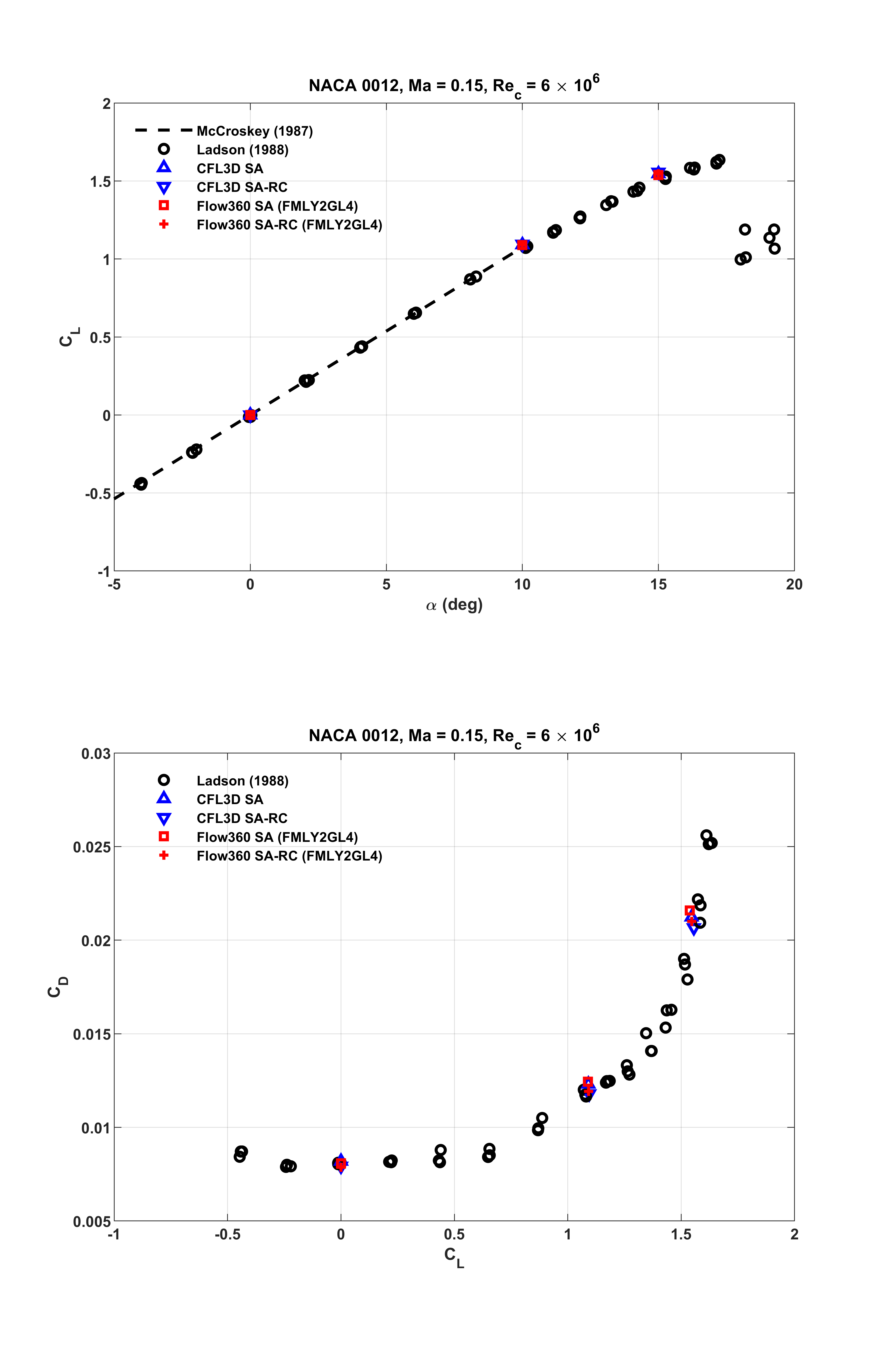
Fig. 5.1.8 Comparisons of \(C_L\) and \(C_D\) at \(\alpha = 0^o\), \(10^o\) and \(15^o\).#
SST(m) Model Results#
Similar to the above sub-section, Flow360 results computed with the SST(m) model are examined in this sub-section. Aerodynamic characteristics were visualized through contour plots of Mach number and turbulent viscosity ratio on the longitudinal cut-plane at \(y = -0.5\). Typical results are shown in Fig. 5.1.9, Fig. 5.1.10 and Fig. 5.1.11 for the three angles of attack, respectively. Similar flow characteristics as discussed earlier are observed.
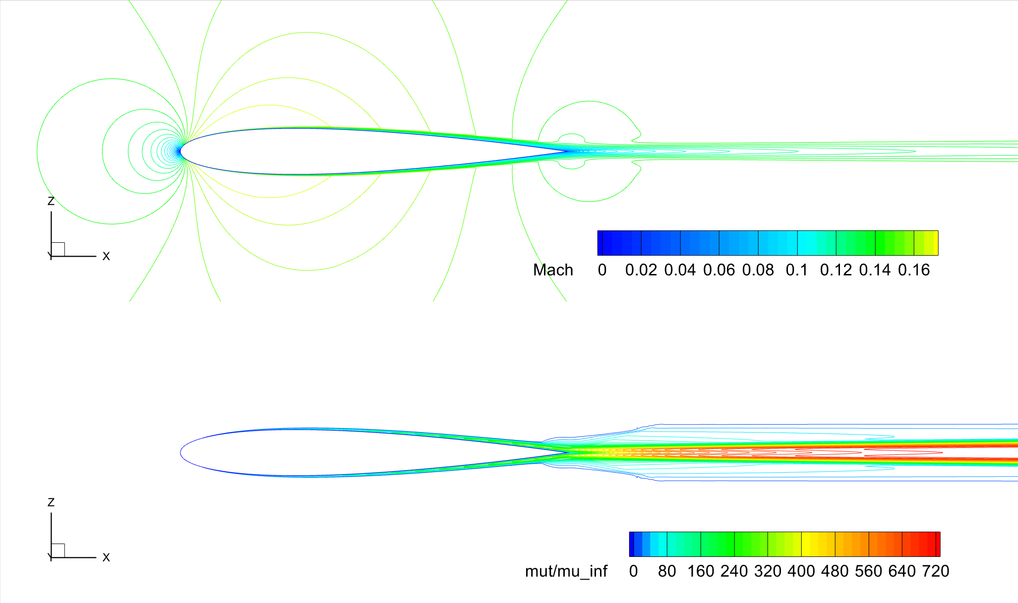
Fig. 5.1.9 Contours of Mach number and turbulent viscosity ratio, NACA 0012, SST(m), \(\alpha = 0^o\).#
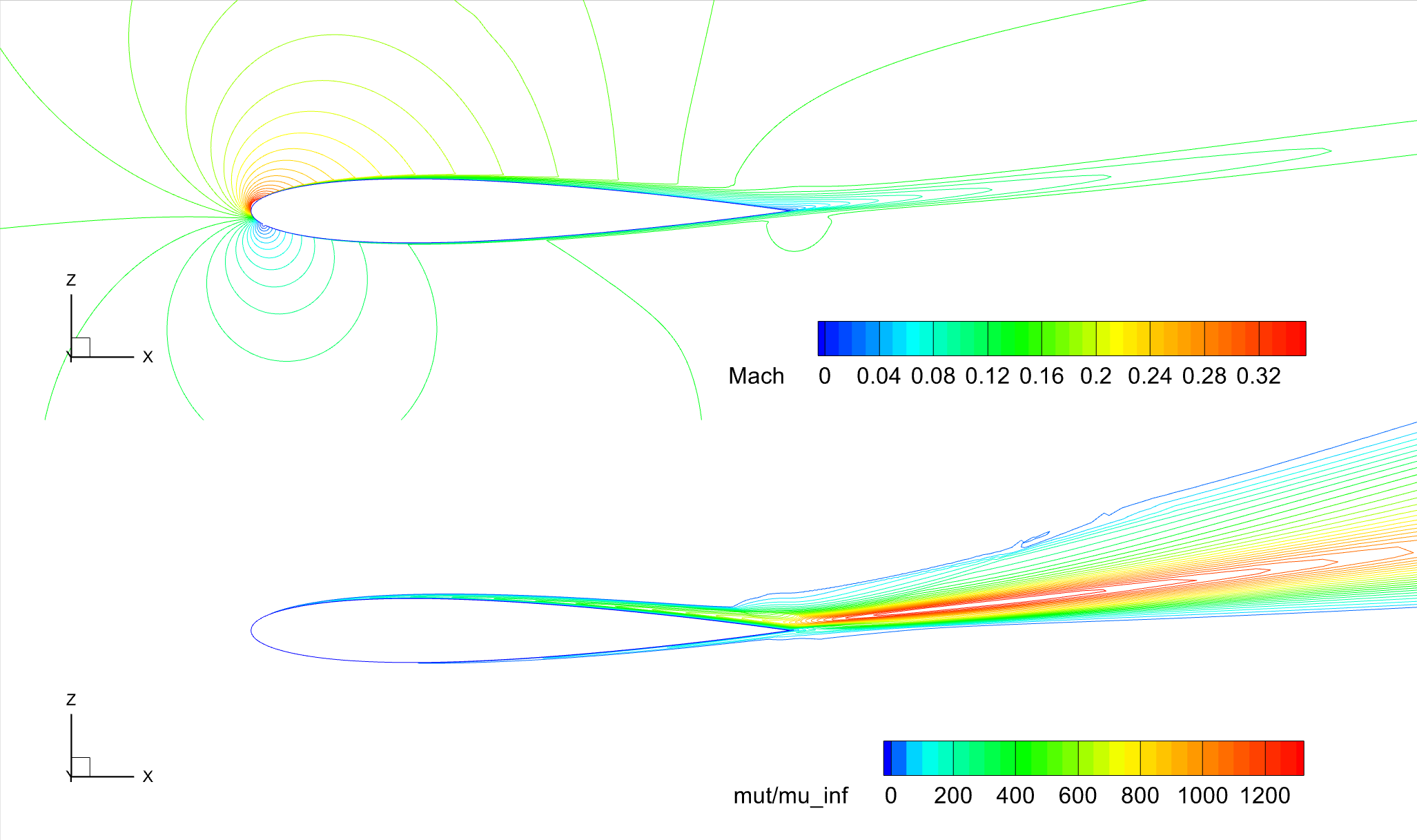
Fig. 5.1.10 Contours of Mach number and turbulent viscosity ratio, NACA 0012, SST(m), \(\alpha = 10^o\).#
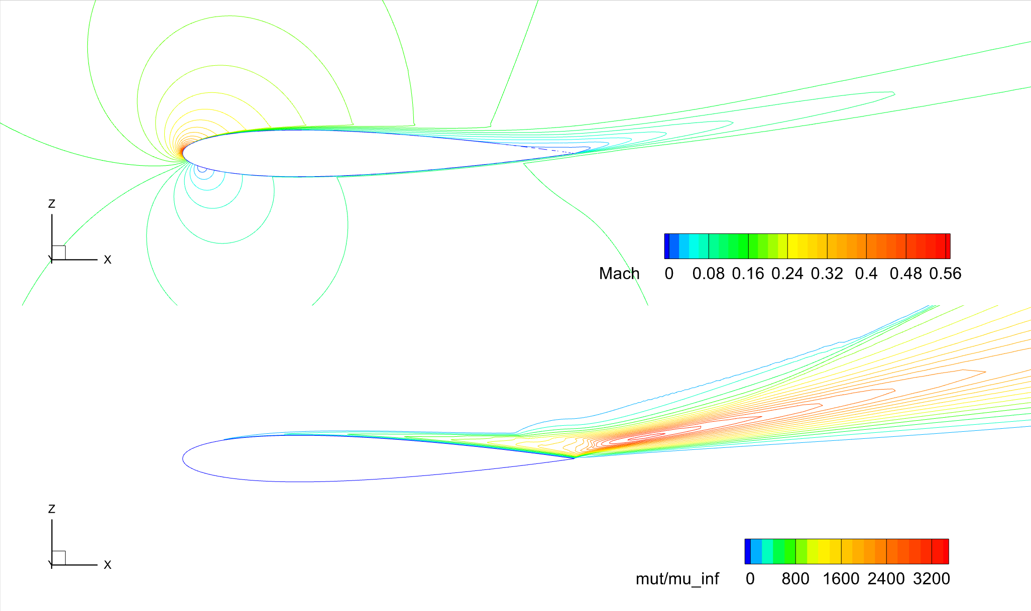
Fig. 5.1.11 Contours of Mach number and turbulent viscosity ratio, NACA 0012, SST(m), \(\alpha = 15^o\).#
For these operating conditions, surface distributions of pressure and skin friction coefficients are examined in Fig. 5.1.12, Fig. 5.1.13 and Fig. 5.1.14, with respect to reference data. In these figures, Flow360 results are indicated as the red solid lines. The corresponding CFL3D results are shown as the blue dashed lines. Also, in these figures, experimental data are given as symbols. These are the same measurements of \(C_p\) made by Gregory and O’Reilly as previously given in Fig. 5.1.5, etc.
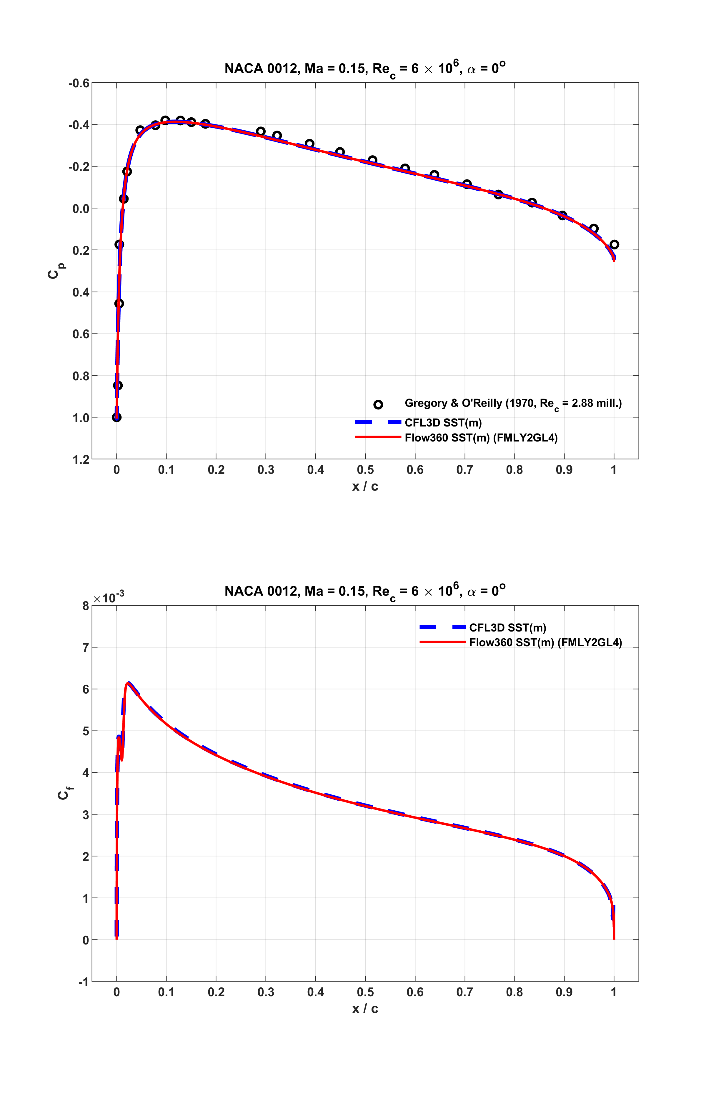
Fig. 5.1.12 Surface distributions of \(C_p\) and \(C_f\), NACA 0012, \(\alpha = 0^o\).#
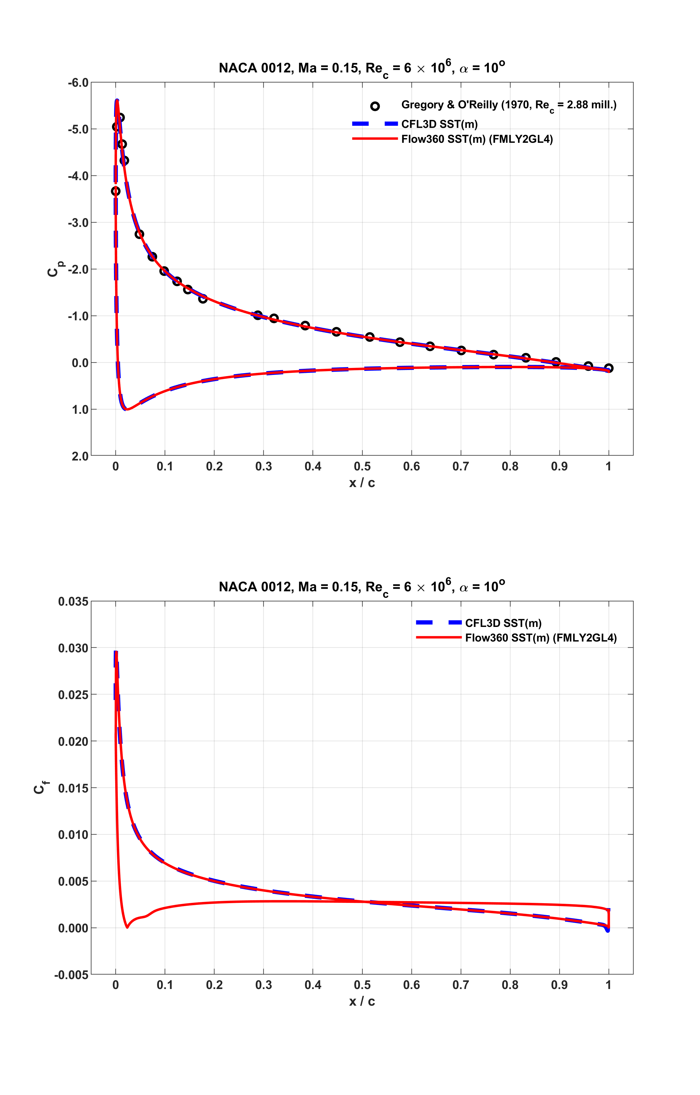
Fig. 5.1.13 Surface distributions of \(C_p\) and \(C_f\), NACA 0012, \(\alpha = 10^o\).#
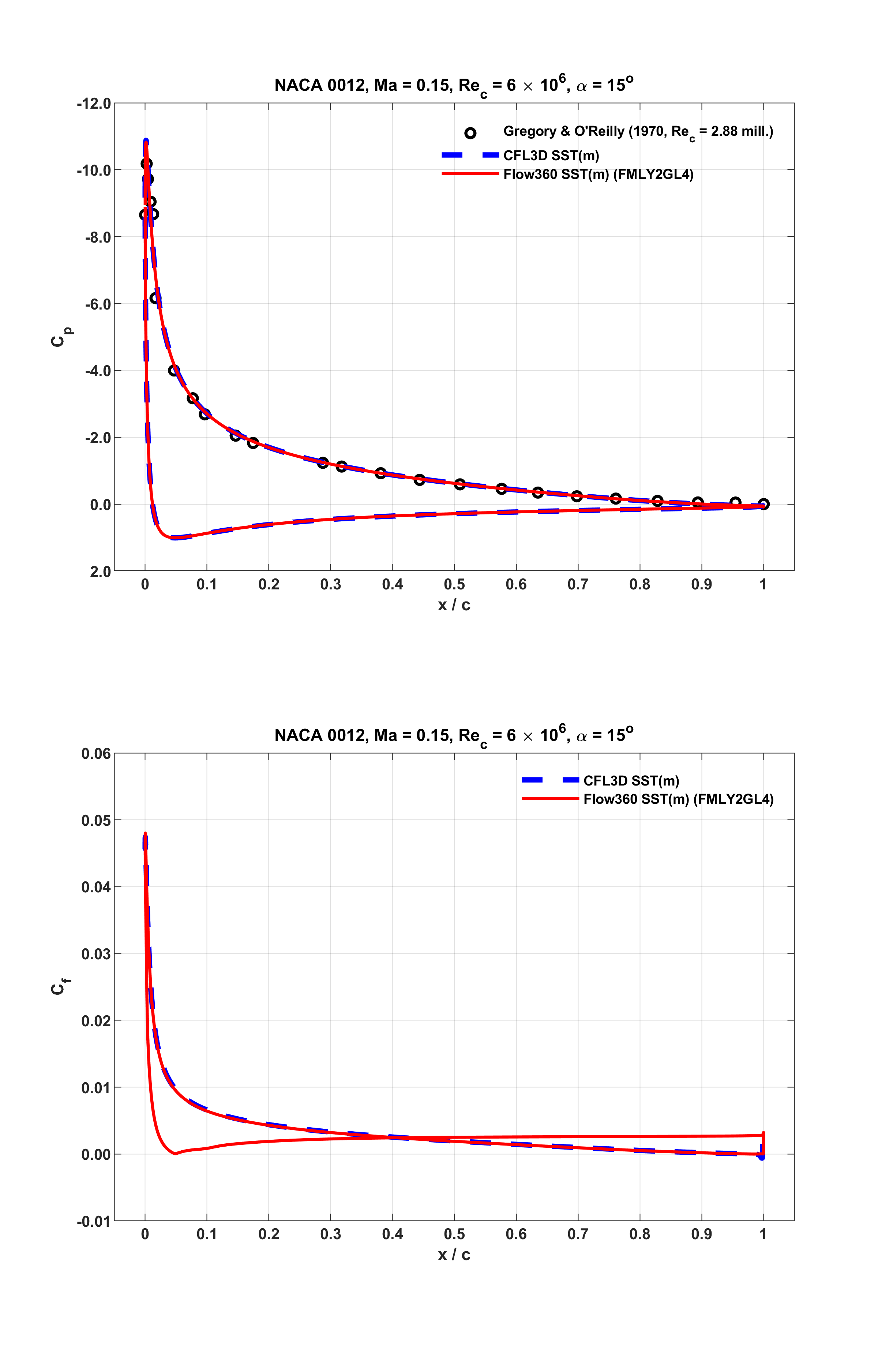
Fig. 5.1.14 Surface distributions of \(C_p\) and \(C_f\), NACA 0012, \(\alpha = 15^o\).#
As seen from the above figures, at all the three distinct lift conditions, Flow360 predictions accurately capture the experimental data, and closely match CFL3D results. Notably, as shown in Fig. 5.1.14 associated with \(\alpha = 15^o\), the \(C_f\) value of the current result with the SST(m) model approaches zero around \(x/c = 0.9834\) on the upper surface of the airfoil near the trailing edge. This indicates separated mean flow occurs as observed from Fig. 5.1.11. For the same operating condition, CFL3D predicted that the separation point emerged around \(x/c = 0.9868\). Similarly, this is located at around \(x/c = 0.9882\) as predicted by OVERFLOW.
The integrated \(C_L\) and \(C_D\) values of the current predictions are summarized in Table 5.1.5, together with available reference CFD data. As seen, for all the tested operating conditions, the accuracy of Flow360 results are comparable. The discrepancies are perhaps attributed to the same aspects as discussed in the previous section.
Codes |
Turb Mdl |
\(\alpha (^o)\) |
\(C_L\) |
\(C_D\) |
\(C_{D,v}\) |
\(C_{D,p}\) |
|---|---|---|---|---|---|---|
CFL3D |
SST(m) |
0 |
-0.763E-05 |
0.00809 |
||
FUN3D |
SST(m) |
0 |
\(\simeq\) 0 |
0.00808 |
||
NTS |
SST(m) |
0 |
\(\simeq\) 0 |
0.00809 |
||
OVERFLOW |
SST |
0 |
\(\simeq\) 0 |
0.00821 |
||
FLOW360 |
SST(m) |
0 |
8.704E-06 |
0.00803 |
0.006724 |
0.001301 |
CFL3D |
SST(m) |
10 |
1.0778 |
0.01236 |
||
FUN3D |
SST(m) |
10 |
1.0840 |
0.01253 |
||
NTS |
SST(m) |
10 |
1.0765 |
0.01251 |
||
OVERFLOW |
SST |
10 |
1.0847 |
0.01262 |
||
FLOW360 |
SST(m) |
10 |
1.0800 |
0.01256 |
0.006141 |
0.006417 |
CFL3D |
SST(m) |
15 |
1.5068 |
0.02219 |
||
FUN3D |
SST(m) |
15 |
1.5109 |
0.02275 |
||
NTS |
SST(m) |
15 |
1.5100 |
0.02187 |
||
OVERFLOW |
SST |
15 |
1.5094 |
0.02288 |
||
FLOW360 |
SST(m) |
15 |
1.5022 |
0.02300 |
0.005222 |
0.017777 |
The corresponding \(C_L\) and \(C_D\) data given in the above table are also displayed in Fig. 5.1.15, together with the experimental data measured by Ladson. Notably, in this figure, at low-to-moderate angles of attack, linear variation of \(C_L\) with the best fit lift slope provided by McCroskey is also shown. As seen, the current results agree well with these references.
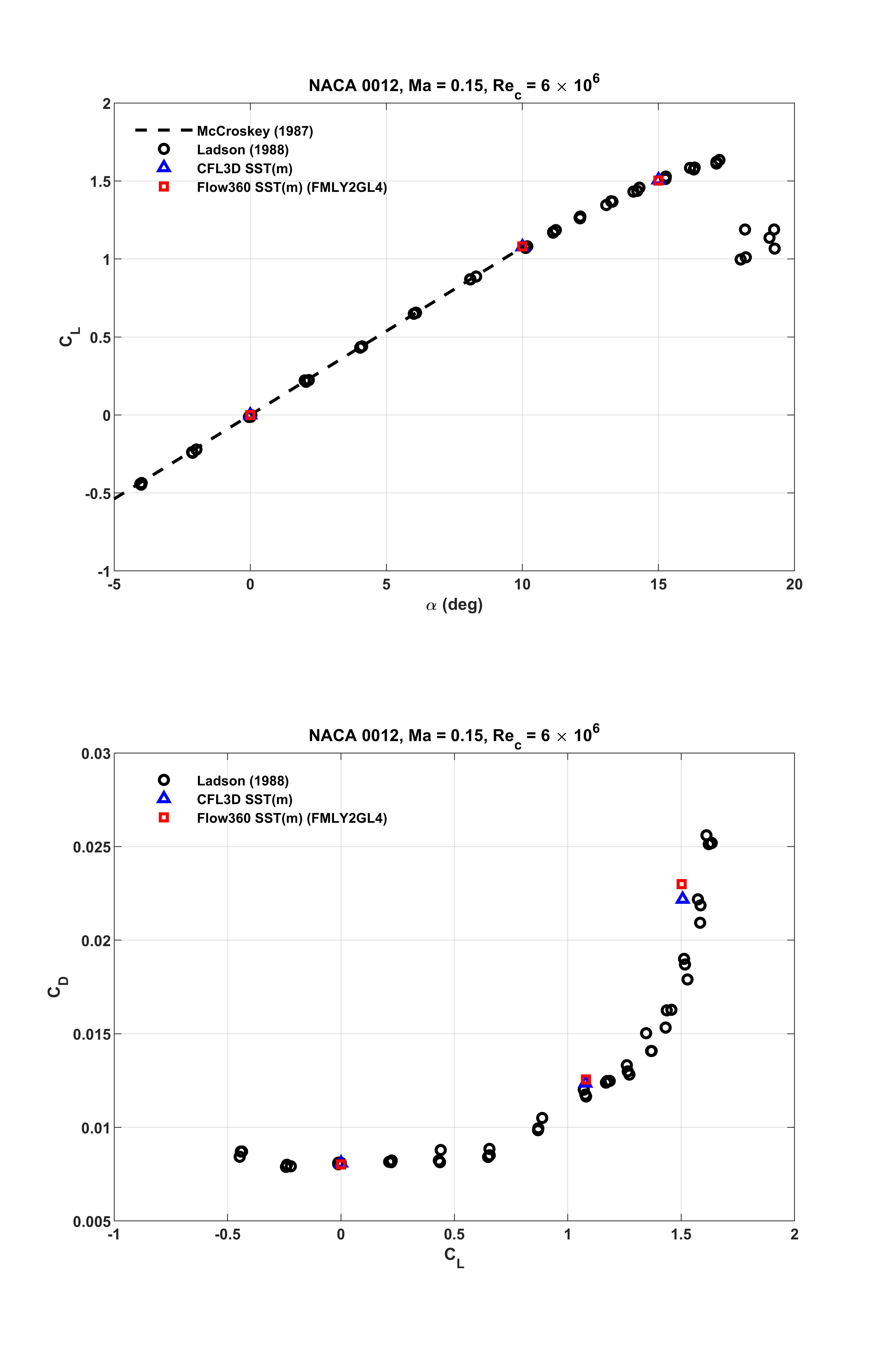
Fig. 5.1.15 Comparisons of \(C_L\) and \(C_D\) at \(\alpha = 0^o\), \(10^o\) and \(15^o\).#
Remarks#
Through this validation study, the flow field, the surface data and the representative aerodynamic quantities predicted by Flow360 were carefully examined. With respect to the latest reference numerical results computed on the same grid as used here, the available agreement on \(C_L\) and \(C_D\) reaches the third significant digit. For the cases with the SA model, the solver version is release-22.1.3.0; where with the SST(m), the same implementation was used as incorporated in the solver of release-22.2.3.0.