5.9. XV-15 Rotor Blade Analysis using the Blade Element Disk Method#
Highlights#
In this case study we are going to show you how to:
Simulate an XV-15 tiltrotor airplane in both hovering helicopter mode and forward flight airplane mode using the steady BET Disk solver in Flow360
Convert nondimensional quantities in the output to dimensional quantities
Introduction#
The development of the XV-15 tiltrotor was launched by the NASA Ames Research Center in collaboration with Bell Helicopters in the late 1960s and early 1970s. It has become the foundation of many VTOL aircrafts today. Unlike typical helicopter rotors, tiltrotor blades demand a compromised design to operate efficiently in both helicopter and propeller modes. Hence, the blades of the XV-15 tiltrotor have high twist, high solidity and small rotor radius. In this case study, we will apply our Blade Element Theory (BET) Model based solver in Flow360 to evaluate the performance of the XV-15 rotor in both helicopter hovering mode and airplane mode.
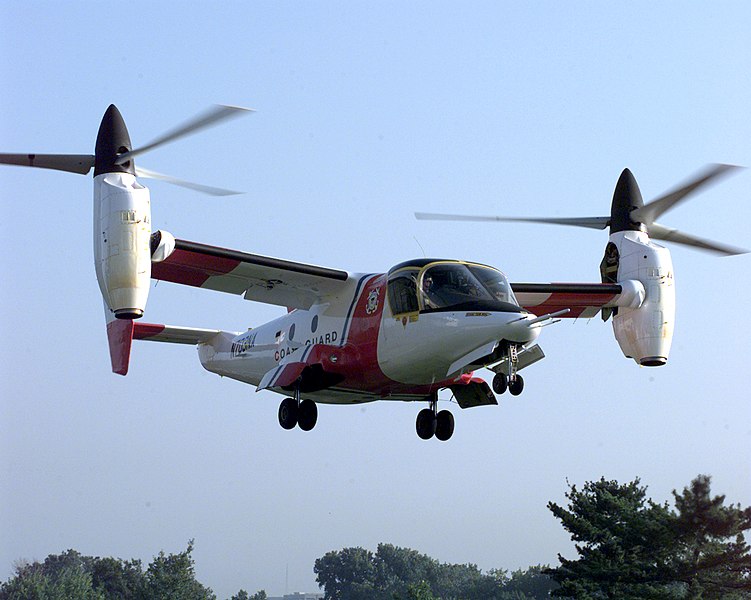
Fig. 5.9.1 The Bell Textron XV-15 Tiltrotor aircraft prepares to land (source: United States Coast Guard)#
The definition of the cross sections of the rotor blade is shown in Table 5.9.1. The main geometric characteristics of the XV-15 rotor blades are listed in Table 5.9.2.
r/R |
Airfoil |
|---|---|
0.09 |
NACA 64-935 |
0.17 |
NACA 64-528 |
0.51 |
NACA 64-118 |
0.80 |
NACA 64-(1.5)12 |
1.00 |
NACA 64-208 |
Parameter |
Value |
|---|---|
Number of blades |
3 |
Rotor radius |
150 inches |
Reference blade chord |
14 inches |
Aspect ratio |
10.71 |
Rotor solidity |
0.089 |
Linear twist angle |
-40.25 degree |
The radial chord and twist distribution is shown in Fig. 5.9.2.
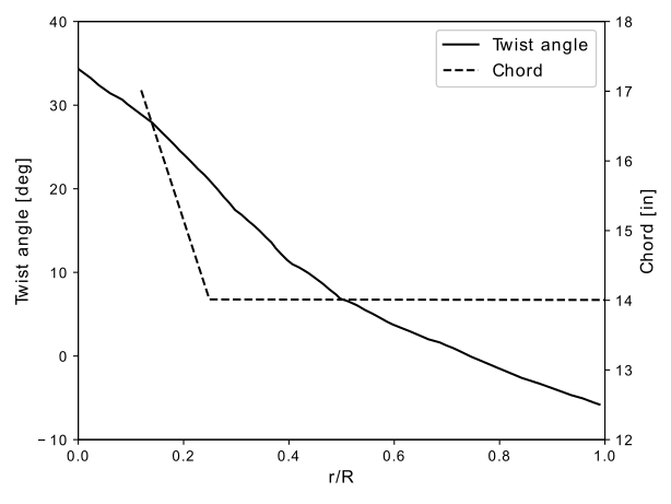
Fig. 5.9.2 XV-15 rotor blade’s twist and chord radial distribution#
More information about the geometry and a high-fidelity detached eddy simulation done using Flow360 can be found at
In this case study, the steady Navier-Stokes solver coupled with the Blade Element Theory Disk method is used to simulate the XV-15 rotor blades under two flight conditions: helicopter hovering mode and airplane mode. In order run cases in a few minutes, compared to the high fidelity unsteady simulations with full rotor geometry in the above paper, the mesh for this BET Disk example is much coarser. The mesh used in the current case study contains only 592K nodes. An overview of a slice of the mesh is shown below
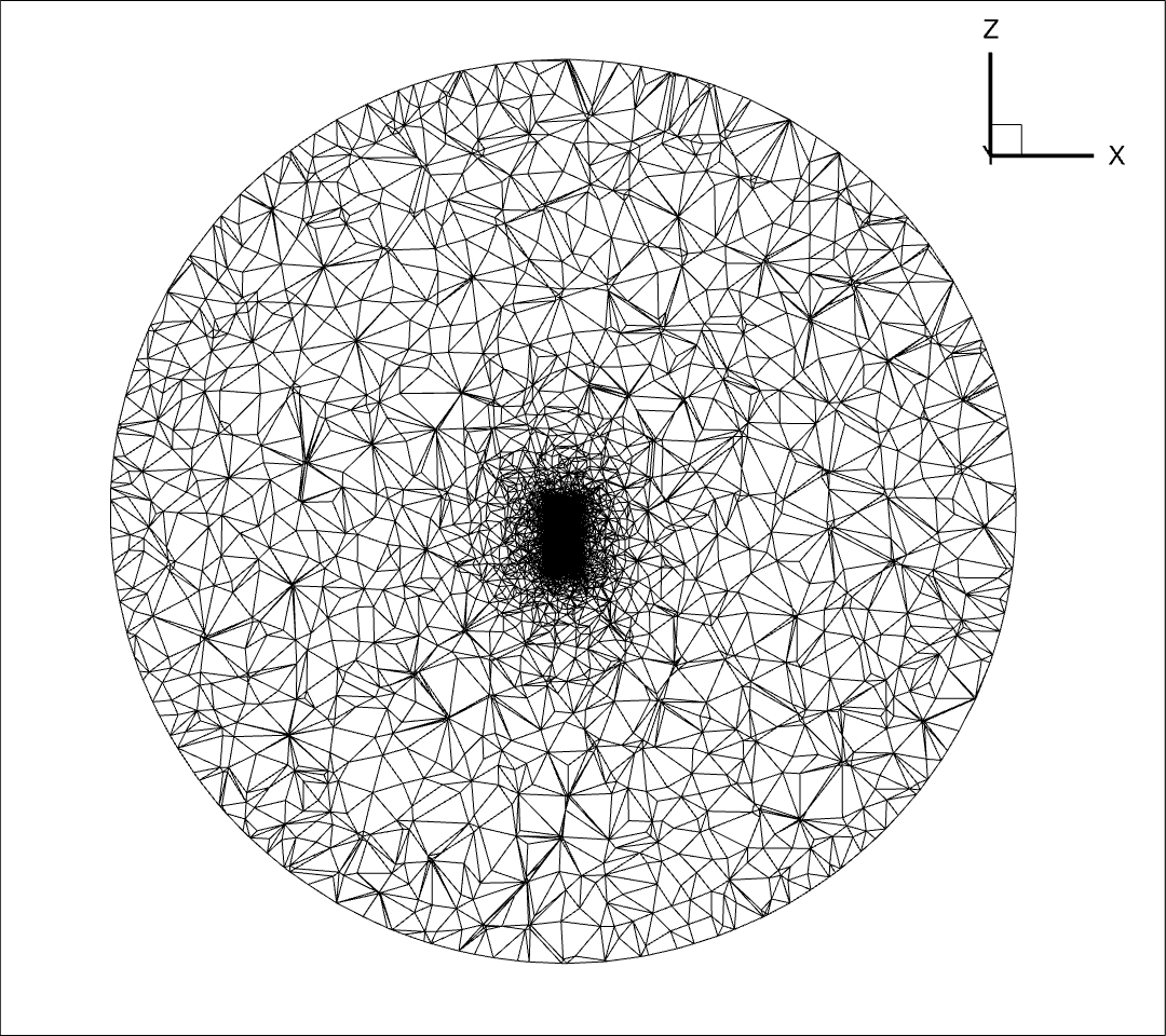
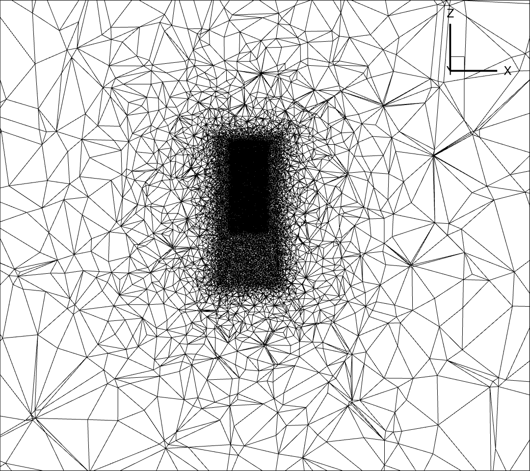
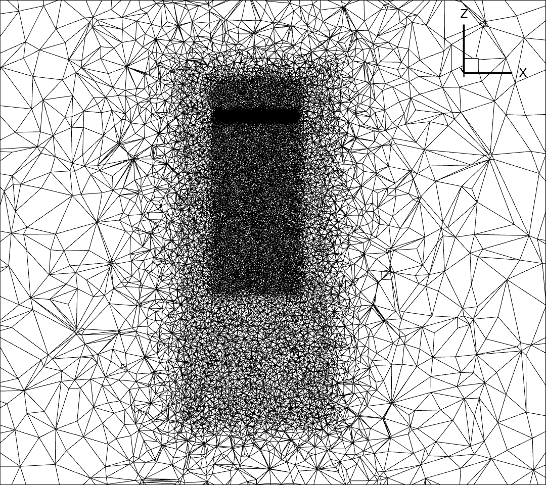
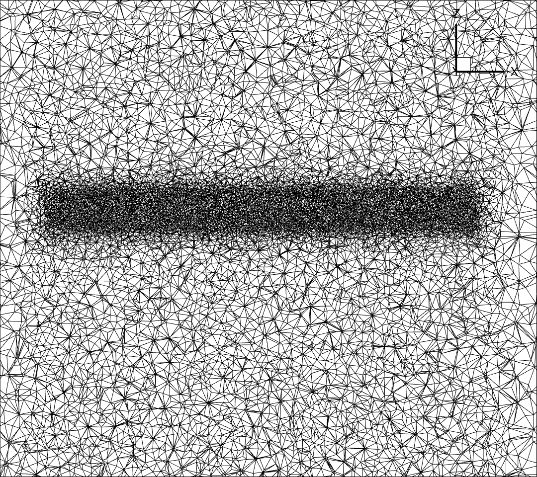
Overview of volume mesh used in BET Disk simulations of XV-15 rotor, successively zooming in from top left->top right->bottom left->bottom right.
The freestream quantities are shown below. These quantities are needed to set up the nondimensional variables in the flow360 case configuration and translate the nondimensional output variables into dimensional values. More information on nondimensionalization in Flow360 can be found at nondim_input and Non-Dimensional Outputs. In the above mesh, the grid unit \(L_{gridUnit}=1\,\text{inch}=0.0254\,\text{meter}\). In this case study, the freestream conditions are set to standard sea level values as shown in Table 5.9.3
air property |
sea level - \(288\,\text{Kelvin}\) |
|---|---|
density, \(\rho_{\infty}\) |
\(1.225\, kg/m^3\) |
speed of sound, \(C_{\infty}\) |
\(340.3\,m/s\) |
Caution
In some simulations, the freestream is not set to be at standard sea level on purpose. For example, in the “case 1a” from 3rd AIAA CFD High Lift Prediction Workshop, the viscosity of the freestream is adjusted to analyze the full-scale geometry at wind tunnel conditions, so please set the freestream properties based on your requirements.
Helicopter Hovering Mode#
In helicopter hovering mode, the freestream velocity is zero. Five blade collective angles are considered in the current study: \(0^o, 3^o, 5^o, 10^o, 13^o\) at \(r/R=0.75\), corresponding to low, medium and high disk loadings. The flow conditions are:
Tip Mach Number, defined as \(U_\text{tip}/C_{\infty}\), is 0.69, so \(U_\text{tip}=0.69C_\infty\).
Reynolds Number (based on reference chord (14 inch) and blade tip speed) = \(4.95\times 10^6\).
Reference Temperature = 288.15 K.
Here are some points to set up the simulation:
Mach number is set to 0, because freestream velocity is zero.
Reference Mach number has to be a non-zero number because the above “Mach” is 0. Theoretically, this value could be arbitrary, but we set it equal to the tip Mach number (0.69) for convenience.
Reynolds number can be calculated as explained below:
The Reynolds number is based on grid unit as the reference length, thus it is mesh dependent. It’s definition is \(\rho_\infty U_\text{ref} L_\text{gridUnit}/{\mu_\infty}\). In the case description, we know the Reynolds number based on tip speed and reference chord is \(4.95\times 10^6\), so we must convert the value from the reference chord used to the \(L_{gridUnit}\) in the mesh.
(5.9.1)#\[\frac{\rho_\infty U_\text{tip} \text{chord}_\text{ref}}{\mu_\infty} = \frac{\rho_\infty \left(0.69 C_\infty\right) \text{chord}_\text{ref}}{\mu_\infty} = 4.95\times 10^6\]
thus the Reynolds number is calculated by:
(5.9.2)#\[\begin{split}\text{reynolds}&=\frac{\rho_\infty U_\text{ref} L_\text{gridUnit}}{\mu_\infty} = \frac{\rho_\infty\cdot \text{MachRef} \cdot C_\infty L_\text{gridUnit}}{\mu_\infty} \\ &=\frac{\rho_\infty \left(0.69 C_\infty\right) \text{chord}_\text{ref}}{\mu_\infty}\times\frac{\text{MachRef}}{0.69}\times\frac{L_\text{gridUnit}}{\text{chord}_\text{ref}} \\ &= 4.95\times 10^6 \times \frac{0.69}{0.69}\times \frac{1\, \text{inch}}{14\, \text{inch}} = 3.3536\times10^5\end{split}\]
The mesh scaled Reynolds number is \(3.3536\times10^5\).
After setting up the case configuration, the case is ready to submit. The 592K-node mesh file can be downloaded via the following link: XV15_BETDisk_R150_592K.lb8.ugrid
Some tips on setting the input quantities related to BET can be found in the BETDisk section of the knowledge base. Please note that there is no hub in the high fidelity detached eddy simulation of the XV-15 rotor blades in our paper mentioned above, so to match the model used in the high fidelity simulations, the chord length in \(r<0.09R\) should be set to 0 in the BET simulation configuration files. I.e. the chord length is set to 0 right before the first cross section (\(r=0.09R\)). This setting leads to a radial distribution similar to “chords_distribution_1” shown in BETDisk.
The forces and moments related to the BET Disk are saved in the “bet_forces_v2.csv” file. A detailed description can be found at Example: BET Loading Output CSV File. Here we will convert those non-dimensional values into dimensional values:
thrust and torque.
Because the axial direction of the rotor is in the Z axis, the thrust is saved as “Disk0_Force_z” and the torque is saved as “Disk0_Moment_z” in the .csv file. The dimensional thrust and torque can be calculated by Eq.(7.1.10) and Eq.(7.1.11):
(5.9.3)#\[\begin{split}\text{Thrust} &= \text{Disk0_Force_z}\cdot \rho_\infty C^2_\infty L^2_\text{gridUnit} \\ &= \text{Disk0_Force_z}\cdot 1.225 kg/m^3 \times 340.3^2 m^2/s^2 \times 0.0254^2 m^2 \\ &= \text{Disk0_Force_z}\cdot 91.5224 N\end{split}\](5.9.4)#\[\begin{split}\text{Torque} &= \text{Disk0_Moment_z}\cdot \rho_\infty C^2_\infty L^3_\text{gridUnit} \\ &= \text{Disk0_Moment_z}\cdot 1.225 kg/m^3 \times 340.3^2 m^2/s^2 \times 0.0254^3 m^3 \\ &= \text{Disk0_Moment_z}\cdot 2.324669 N\cdot m\end{split}\]
The convergence history of the dimensional thrust and torque using steady BET Disk solver is shown in following figures:


Loading convergence of BET Disk simulation in hovering helicopter mode at various pitch angles.
sectional thrust and torque.
In the “bet_forces_v2.csv” file, the sectional thrust coefficients are provided. The process to convert the nondimensional Ct into its physical dimension, i.e. sectional thrust per unit span in SI is very similar to the one shown above. We need the dimensional quantities mentioned in Eq.(7.1.12) and Eq.(7.1.13) to compute the dimensional sectional thrust:
Radius of the rotor disk \(R = 150\times L_{gridUnit} = 3.81\,\text{meter}\)
rotating angular speed \(\Omega = V_{tip}/R = Mach_{tip}*C_{\infty}/R = 61.6237\, \text{rad/second}\)
reference chord \(\text{chord}_{\text ref}=14\times L_{gridUnit} = 0.3556\, \text{meter}\)
If we assume that we want to calculate the sectional thrust and torque at the first disk’s first blade’s second radial location, i.e. Disk0_Blade0_R1:
As a comparison example between the high fidelity full-rotor unsteady simulation and the BET Disk steady simulation, the physical sectional thrust on a blade per unit span, for the \(\theta_{75}=10^o\) case, is shown below


Sectional thrust distribution and history of total thrust in hovering mode, \(\theta_{75}=10^o\).
The biggest differences between these high fidelity simulations and these BET Disk simulations are near the tip regions where blade-vortex interactions are strong. The flow around the tip can be highly three dimensional, making a BET Disk approximation locally inaccurate. This effect is proportional to the blade disk loading, thus it is larger at hovering or near-hovering conditions when the thrust is higher then in forward flight. Even then, the total thrust of the three blades in hover, compared to the Flow360 high fidelity unsteady simulation, is ~8% different. This level of accuracy makes the BET Disk a useful tool in the preliminary design stages.
To provide another overview of the BET disk accuracy; If we look at the propeller efficiency in hovering mode, the thrust coefficient, the torque coefficient and the figure of merit defined in Eq.(5.9.6) and compare them with several experimental data and numerical prediction of high-fidelity DES simulations, we get the graphs below:
where \(R\) is rotor disk radius and \(A\) is rotor disk area, i.e. \(\pi R^2\)


Comparison on thrust and torque coefficient and figure of merit in hovering mode at various pitch angles.
Airplane Mode#
In airplane mode, four blade collective angles are considered: \(26^o, 27^o, 28^o, 28.8^o\) at \(r/R=0.75\). The flow conditions are:
Tip Mach Number = 0.54.
Reynolds Number (based on reference chord and tip speed, with no account for the inflow velocity) = \(4.5\times 10^6\).
Reference chord = 14 inch.
Reference Temperature= 288.15 K.
Advance ratio (defined as inflow speed over tip speed) = 0.337
The mesh file is the same as the files used in the helicopter hovering example above.
The convergence history of the thrust coefficients and torque coefficients using the steady BET Disk solver are shown below


Convergence history of thrust coefficient and torque coefficient in airplane mode at various pitch angles.
As an example, similarly to the helicopter hovering case shown above, the physical sectional thrust for the \(\theta_{75}=26^o\) case is shown below. We have comparisons to the high fidelity DES simulation both on a blade per unit span basis and for the total force.
Note
Please note the non-zero origin of the Y axis on the right plot of total force.


Sectional thrust distribution and thrust history in airplane mode at \(\theta_{75}=26^o\).
To provide an overview of power efficiency in airplane mode at various pitching angles, the figure below shows the comparison of the thrust coefficient, torque coefficient and propeller propulsive efficiency, defined in Eq.(5.9.7), between the BET Disk and high fidelity simulations.


Comparison of thrust coefficient, torque coefficient and propulsive efficiency in airplane mode at various pitch angles.