5.5. Wall Model#
Introduction#
This case study presents and validates the wall model implemented within Flow360. Wall model simulations offer significant advantages over wall-resolved simulations leading to reductions in computational cost and speed improvements with limited impact on the simulation accuracy. Wall-resolved simulations typically require a \(y^+\) on the order of 1 and a significant number of points in the boundary layer, to correctly capture boundary layer profile and shear stress on the wall. Wall model simulations use an analytical nonlinear function in this region across the first cell, meaning that the first cell spacing can be significantly larger. This leads to a reduction in the mesh size, but also improved simulation convergence properties as the smallest cell volume in the mesh, which is typically in the boundary layer, is much larger. The larger smallest edge length also allows for meshing of CAD models with greater geometric tolerances. The wall model in Flow360 differs from typical wall model implementations, with the formulation described in the next section. The wall model is demonstrated for five cases: the zero pressure-gradient flat plate, the NACA0012 aerofoil, the OM6 wing, the Ahmed body and the Windsor body. For each of the cases, a number of wall spacings were simulated for both the Spalart-Allmaras and \(k-\omega\) SST turbulence models. The main purpose of this study is validation of the wall model in Flow360 and recommendations on the most optimal wall spacing in terms of computational cost and accuracy.
Wall Model Formulation in Flow360#
The wall model formulation in Flow360 is based on the concept of a wall velocity. Both the velocity at the wall and at the first grid point are updated during the solution process. From the solution, the ratio between the tangential velocities at the wall and first grid point is obtained (\(U_0/U_1\)). Then we define the laminar and turbulent shear stresses as a function of the velocity ratio, with the total shear stress being the sum of the laminar and turbulent contributions. The \(y^+\) value is then obtained from the wall shear stress. To determine the accuracy of the wall model, a wallFunctionMetric can be output as part of the surface solution, with values below 1.25 indicating good estimation of the wall shear stress and values of above 10 meaning an unreliable estimation.
Flat Plate Case#
Simulation Setup#
The first case under consideration is the flat plate case, which is a canonical case often used for testing new implementations in CFD. The flat plate case is based on the model verification case available on the NASA TMR website. The freestream Mach number is equal to 0.2 with the Reynolds number per unit length equal to 5 million. The boundary conditions applied are based on the Flat Plate TMR Case, with the NoSlipWall boundary condition replaced with WallFunction for the wall model cases. The grids were generated based on the 137 by 97 nodes grid from the NASA TMR flat plate grids download page. This grid was loaded into a meshing tool and the wall spacing was modified to a number of values ranging from 4e-07 to 2e-03 to examine the effect of different \(y^+\) values on the results. The wall resolved and wall model grids for a target \(y^+\) value of 100 are compared in Fig. 5.5.1.
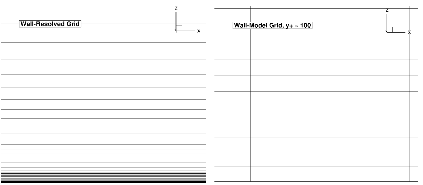
Fig. 5.5.1 Comparison of the wall-resolved (top) and wall-model (\(y^+\) ~100 (bottom) grids for the flat plate case.#
As the number of points in the wall normal direction is fixed, the wall-model grid has a finer spacing away from the boundary layer due to the higher wall-normal spacing at the flat plate. The simulations were performed using both the Spalart-Allmaras and \(k-\omega\) SST turbulence models. The CFL number was ramped up from 1 to 500 over 2000 pseudo-steps with a total number of pseudo-steps equal to 5000.
Numerical Results#
Firstly, the drag values are compared across a range of wall spacings, shown in Table 5.5.1. The same data is shown in graphical format in Fig. 5.5.2.
Wall Spacing |
\(y+\) (Spalart-Allmaras, x=1.0) |
CD (Spalart-Allmaras) |
CD (\(k-\omega\) SST) |
|---|---|---|---|
1E-06 (resolved) |
0.182 |
0.002846 |
0.002826 |
1E-06 |
0.176 |
0.002670 |
0.002654 |
4E-06 |
0.693 |
0.002581 |
0.002528 |
2E-05 |
3.25 |
0.002257 |
0.002139 |
4E-05 |
6.25 |
0.002077 |
0.001928 |
0.0001 |
16.3 |
0.002292 |
0.002090 |
0.0002 |
34.5 |
0.002544 |
0.002247 |
0.0004 |
68.3 |
0.002497 |
0.002398 |
0.0008 |
134 |
0.002423 |
0.002552 |
0.002 |
331 |
0.002373 |
0.002633 |
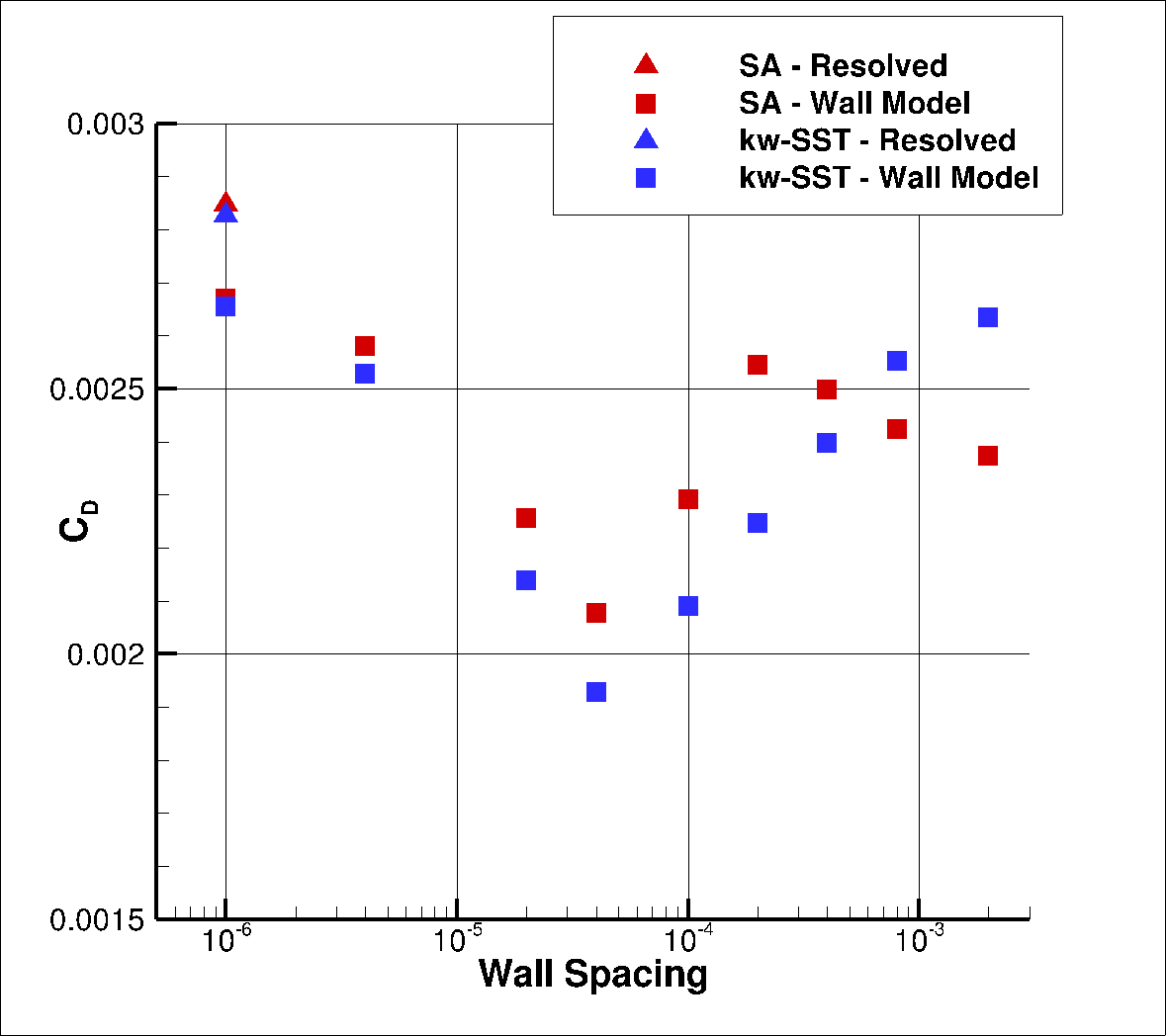
Fig. 5.5.2 Drag values for the flat plate case for a range of wall spacings for the Spalart-Allmaras and \(k-\omega\) SST turbulence models.#
As the wall spacing increases, the drag value is minorly underpredicted compared to the wall-resolved simulations, with the difference staying within 10% for the first two wall spacings. As the wall spacing is increased further, the error on the drag prediction increases, until spacings of 0.0002-0.0004 are reached, above which the error significantly reduces. Similar trends are observed between the Spalart-Allmaras and \(k-\omega\) SST turbulence models, although the error on the drag prediction appears to be slightly higher for the \(k-\omega\) SST turbulence model across nearly all wall spacings. At very high wall spacings, the \(k-\omega\) SST model appears to perform better than the Spalart-Allmaras model. To analyse these findings further, we first look at the \(y+\) and skin friction distributions, shown in Fig. 5.5.3-Fig. 5.5.4. A boundary layer profile in wall units according to the Law of the wall is also shown in Fig. 5.5.5 to aid the discussion.
.svg)
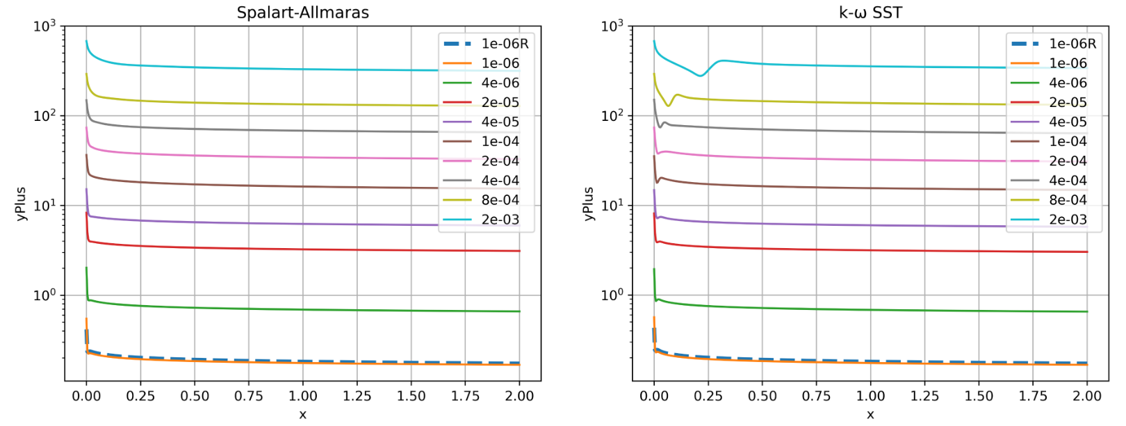
Fig. 5.5.3 Y+ values along the flat plate for wall-resolved (R) and wall-model simulations for the Spalart-Allmaras and \(k-\omega\) SST turbulence models.#
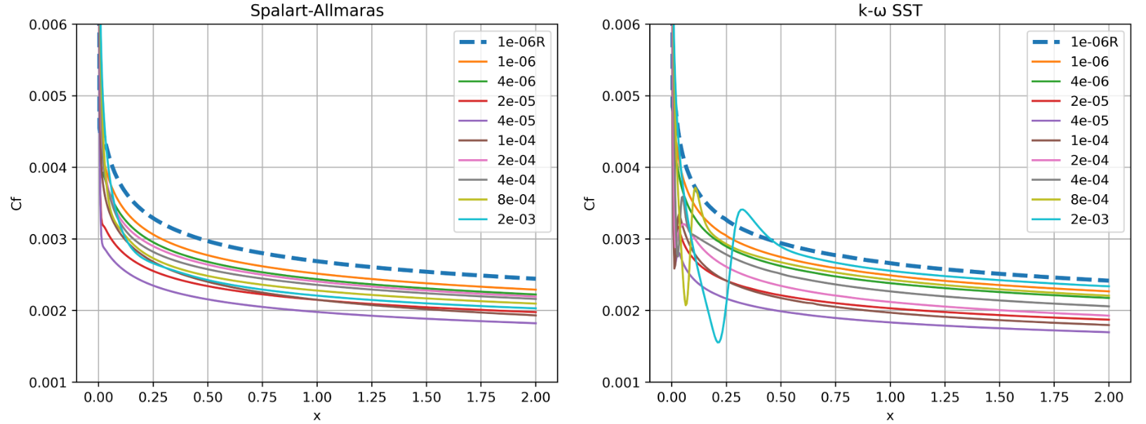
Fig. 5.5.4 Skin friction predictions along the flat plate for wall-resolved (R) and wall-model simulations for the Spalart-Allmaras and \(k-\omega\) SST turbulence models.#
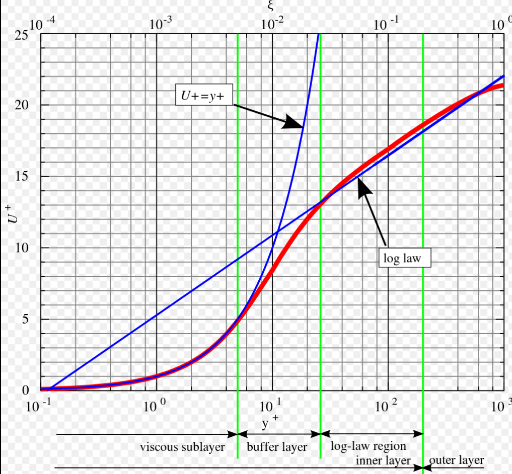
Fig. 5.5.5 Boundary layer profile in wall units according to the Law of the wall.#
The first observation is that the spacings with poorest agreement in drag have \(y^+\) values ranging from 5 to 30. This region corresponds to the buffer layer of the boundary layer, where viscous and turbulent stresses are of similar magnitude. For a boundary layer profile in wall units, this is where a linear function in the viscous sublayer moves into the log-law region. Therefore, if the first cell height is in the buffer layer, as with other wall function implementations, poorer agreement with a resolved simulation will be obtained. The spacings of 0.0002 and 0.0004 where good agreement was obtained with the resolved simulation lie in the \(y^+\) range of 50 to 100. Similar profiles are obtained for the \(k-\omega\) SST turbulence model, although a dip in the \(y^+\) values in seen at higher wall spacings. Similar curve gradients are obtained for the Spalart-Allmaras cases between the wall-resolved and wall-model simulations, apart from the two highest wall spacings where the gradient near the start of the plate is much shallower. For the \(k-\omega\) SST turbulence model similar observations can be made, although, the two highest wall spacings appear to behave like transitional calculations, which is incorrect for a fully-turbulent simulation. The production of turbulence appears to be delayed for \(k-\omega\) SST wall model simulations with high \(y^+\) values. To further analyze the results, we extract the velocity and turbulent eddy viscosity ratio profiles at x=0.98, shown in Fig. 5.5.6 and Fig. 5.5.7
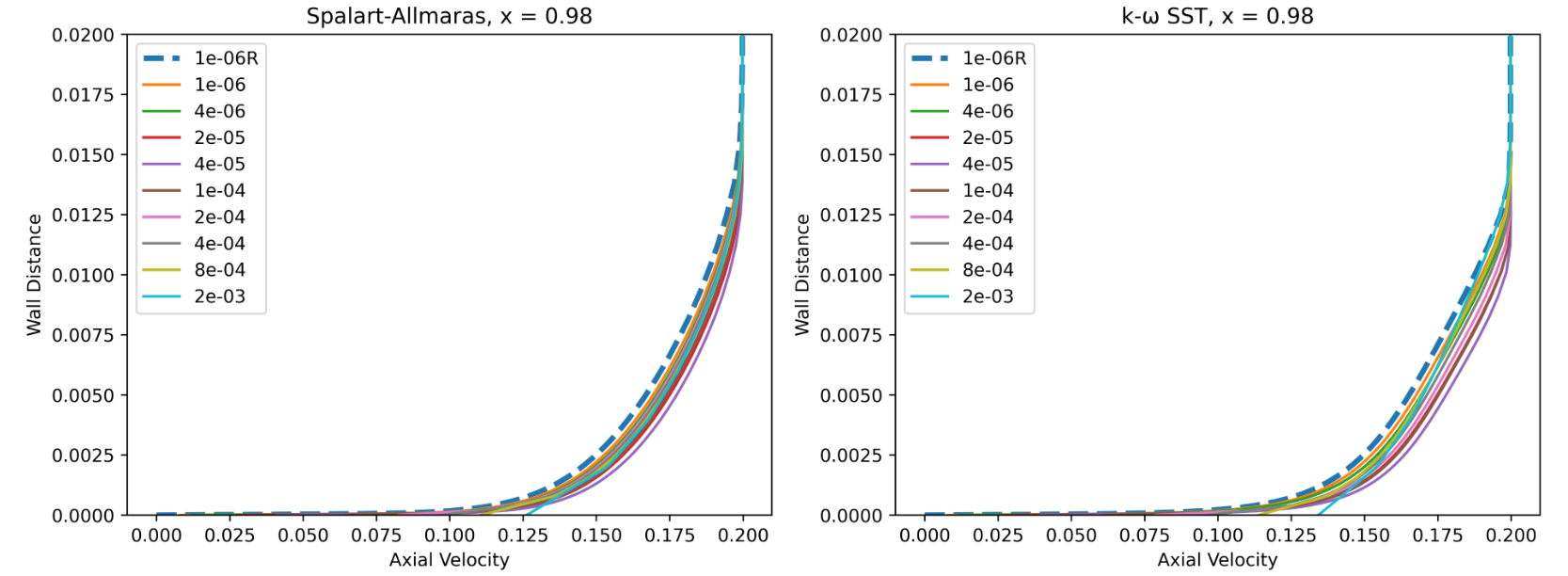
Fig. 5.5.6 Velocity profiles at x = 0.98 for wall-resolved (R) and wall-model simulations for the Spalart-Allmaras and \(k-\omega\) SST turbulence models.#
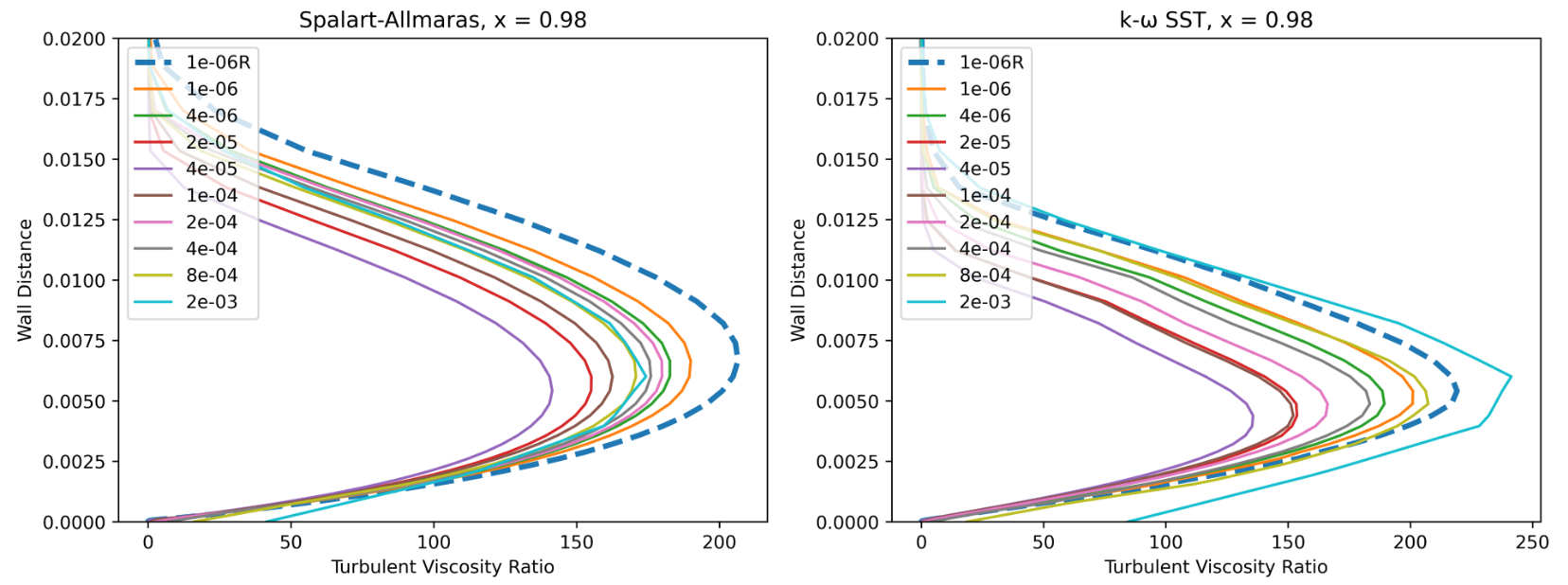
Fig. 5.5.7 Turbulence viscosity ratio at x = 0.98 for wall-resolved (R) and wall-model simulations for the Spalart-Allmaras and \(k-\omega\) SST turbulence models.#
The first observation is that for the wall model simulations, the axial velocity is non-zero at the wall as discussed in the wall model formulation. Very good agreement is obtained for the velocity profiles across a range of wall spacings, with the wall model simulations predicting a slightly higher velocity magnitude in the boundary layer. The poorest agreement is seen for wall spacings which are equivalent to the first layer thickness being in the buffer layer. Comparing the Spalart-Allmaras and \(k-\omega\) SST results, it can be seen that the velocity increase is more linear for the \(k-\omega\) SST model. The turbulent eddy viscosity ratio profiles, are also well resolved by the wall model simulations. The peak eddy viscosity ratio is typically slightly underpredicted although wall spacings of 2e-04 and 4e-04 give reasonably good agreement with the wall-resolved simulations. Similar peak values are predicted by the Spalart-Allmaras and \(k-\omega\) SST turbulence model simulations, although the \(k-\omega\) SST predictions lead to a sharper profile. The profile is slightly underesolved for the highest wall spacing. Since, only the first layer height is changed in the mesh with a constant growth rate, high wall spacings also lead to a coarser mesh across the boundary layer. This is why a discontinuous curve is seen at the highest wall spacing of 2e-03. A more qualitative comparison of the turbulent eddy viscosity ratio profiles is shown in Fig. 5.5.8 for wall-resolved simulations and the wall-model simulation with a wall spacing of 4e-04.
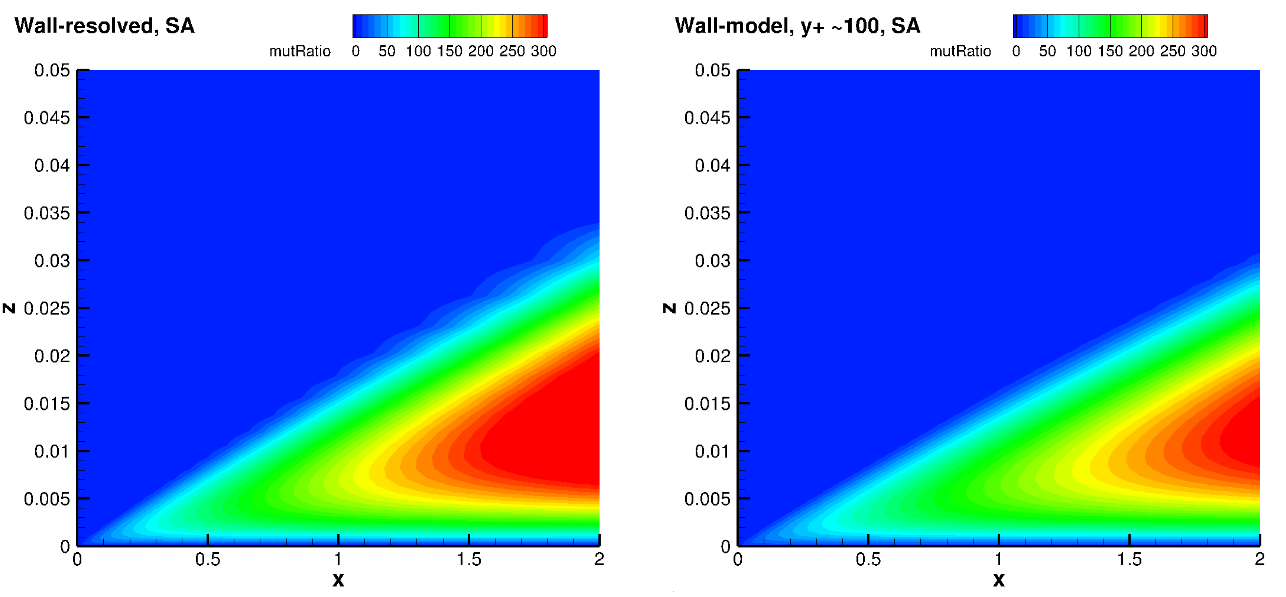
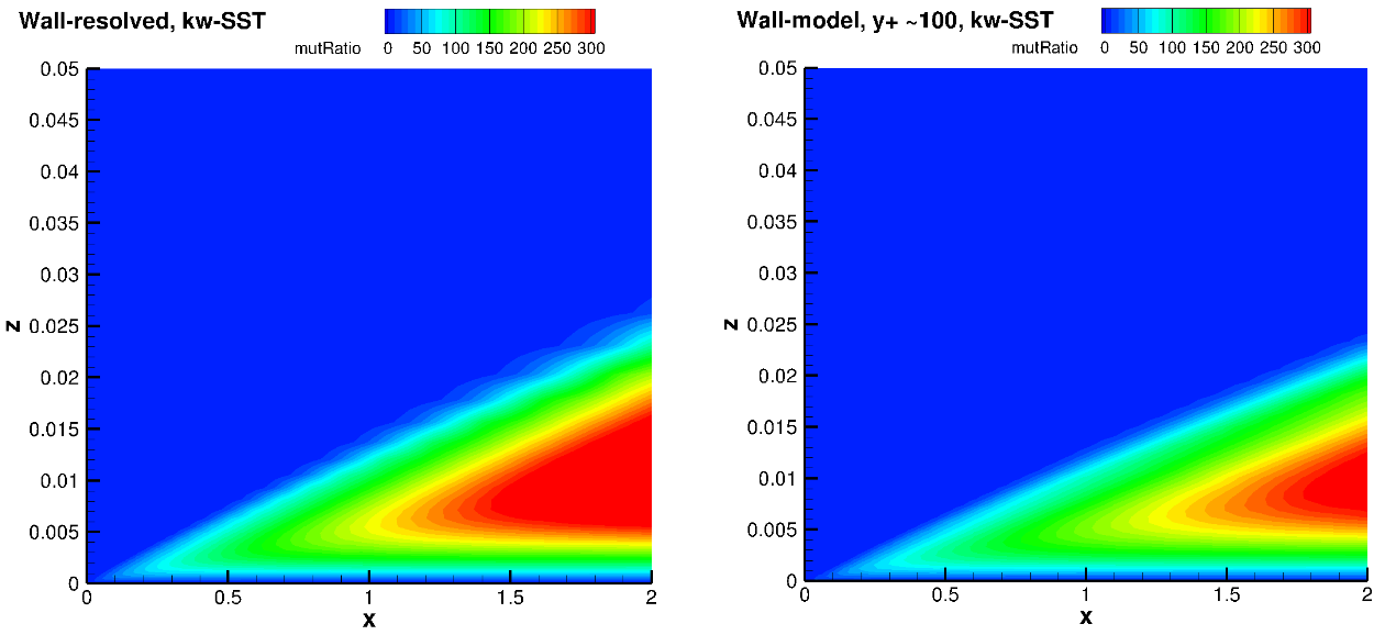
Fig. 5.5.8 Turbulence viscosity ratio fields for the wall-resolved (left) and wall-model at a \(y+\) ~100 (right) simulations for the Spalart-Allmaras and \(k-\omega\)-SST turbulence models.#
The turbulence eddy viscosity ratio fields show similar trends between wall-resolved and wall-model simulations. The peak eddy viscosity ratio is generally lower in the domain for the wall model simulations. The growth of eddy viscosity in the wall normal direction is lower for the \(k-\omega\) SST model when compared to the Spalart-Allmaras turbulence model.
NACA0012 Case#
Simulation Setup#
The second case under consideration is the NACA0012 aerofoil at three angles of attack of \(0^o\), \(10^o\) and \(15^o\). The main purpose of this case is to test the wall model for a case that is closer to aerospace applications, and examine the effect of pressure gradients on the accuracy of the wall model. The NACA0012 case is another model verification case available on the NASA TMR website. We have verified our wall-resolved simulations for this case in the NACA0012 case study. For reference, the Reynolds number for this case is 6 million with a Mach number of 0.15. In the present case study, we examine the same case across a range of wall spacings. The grids were generated using our automated meshing workflow Automated Meshing. The surface grid is fixed with 513 points on the surface, corresponding to the Level 4 grid on the NASA TMR NACA0012 grids downloads page. The volumetric grid was generated automatically, with wall spacings varying from 5e-07 to 0.001, leading to node counts of 59,654 to 19,488. This means that the grid with the highest wall spacing has less then a third of the nodes. One cell (Two nodes) is used in the spanwise direction. The wall resolved and wall model grids for a target \(y^+\) value of 100 are compared in Fig. 5.5.9.
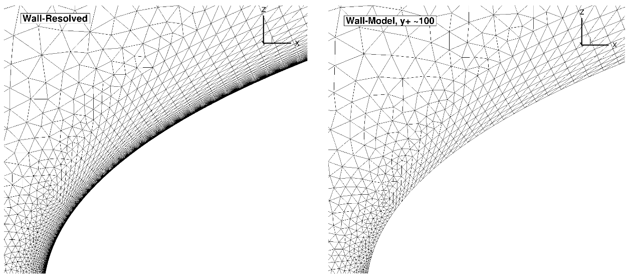
Fig. 5.5.9 Comparison of the wall-resolved (left) and wall-model (\(y^+\) ~100 (right) grids for the NACA0012 case.#
The volumetric grids for the wall-resolved and wall-model grids look fairly similar when looking at the grid around the entire aerofoil. The wall-model grid for a \(y^+\) of the 100, however, has fewer anisotropic layers, leading to a node count of 26,180 nodes (resolved grid is 59,654). The means that the computational cost on the wall-model grid will be less then half (additionally convergence will be faster due to a larger minimum volume). The simulations were performed using both the Spalart-Allmaras and \(k-\omega\) SST turbulence models. The CFL number was ramped up from 5 to 200 over 2000 pseudo-steps with a total number of pseudo-steps equal to 10000, even though in many cases, fewer pseudo-steps could have been used.
Numerical Results#
Firstly, the integrated loads are compared for wall-resolved and wall-model simulations. The integrated loads at an angle of attack of \(0^o\) are shown in Table 5.5.2 for both examined turbulence model, with the same data shown in graphical format in Fig. 5.5.10.
Wall Spacing |
CL (Spalart-Allmaras) |
CL (\(k-\omega\) SST) |
CD (Spalart-Allmaras) |
CD (\(k-\omega\) SST) |
|---|---|---|---|---|
5E-07 (resolved) |
-0.0000358 |
-0.0000099 |
0.0081878 |
0.0082157 |
5E-07 |
-0.0000381 |
-0.0000148 |
0.0076578 |
0.0076832 |
2E-06 |
-0.0004925 |
-0.0005105 |
0.0074463 |
0.0073613 |
1E-05 |
-0.0002107 |
-0.0001959 |
0.0067913 |
0.0064732 |
2E-05 |
-0.0004692 |
-0.0004715 |
0.0062709 |
0.0058601 |
5E-05 |
-0.0003264 |
-0.0004367 |
0.0062592 |
0.0055318 |
0.0001 |
-0.0001271 |
-0.0001083 |
0.0072587 |
0.0060029 |
0.0002 |
-0.0000014 |
0.0000725 |
0.0074976 |
0.0062179 |
0.0004 |
0.0001888 |
0.0001342 |
0.0073109 |
0.0061955 |
0.001 |
-0.0003806 |
-0.0006551 |
0.0075675 |
0.0067801 |
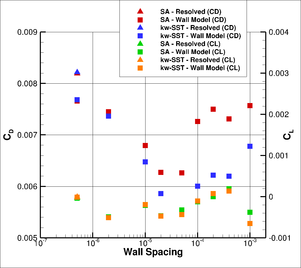
Fig. 5.5.10 Integrated loads values for the NACA0012 case at \(0^o\) for a range of wall spacings for the Spalart-Allmaras and \(k-\omega\) SST turbulence models.#
At an angle of attack of \(0^o\) the lift coefficient should be zero for a symmetrical airfoil. Here, the lift coefficient is nearly zero for the resolved simulation, with errors due to the unstructured nature of the grid (top and bottom side of the airfoil will have a slightly different grid). For wall model simulations, the lift coefficient in most cases has a slightly higher magnitude, however, the values can still be approximated to zero. For the drag prediction, just like for the flat plate case above, a minor error of under 10% can be seen at low wall spacings, with the error increasing as the spacing is increased to about the buffer layer thickness and then the error reduces as the first layer thickness continues to increase. The wall-model simulations seem to have better agreement with the wall-resolved simulations with the Spalart-Allmaras turbulence model when compared to the \(k-\omega\) SST model. The integrated loads at a higher angle of attack of \(10^o\) are shown in Table 5.5.3 and Fig. 5.5.11.
Wall Spacing |
CL (Spalart-Allmaras) |
CL (\(k-\omega\) SST) |
CD (Spalart-Allmaras) |
CD (\(k-\omega\) SST) |
|---|---|---|---|---|
5E-07 (resolved) |
1.0884010 |
1.0887404 |
0.0134051 |
0.0135129 |
5E-07 |
1.0954417 |
1.0961686 |
0.0125759 |
0.0126426 |
2E-06 |
1.0990507 |
1.1015714 |
0.0122834 |
0.0121173 |
1E-05 |
1.1111295 |
1.1166378 |
0.0110191 |
0.0104134 |
2E-05 |
1.1162736 |
1.1237324 |
0.0104958 |
0.0095929 |
5E-05 |
1.1099161 |
1.1213013 |
0.0112073 |
0.0098585 |
0.0001 |
1.0975726 |
1.1083656 |
0.0127432 |
0.0115825 |
0.0002 |
1.0891533 |
1.0946613 |
0.0137239 |
0.0133125 |
0.0004 |
1.0724442 |
1.0741733 |
0.0146291 |
0.0147813 |
0.001 |
1.0221160 |
1.0127430 |
0.0169448 |
0.0177315 |
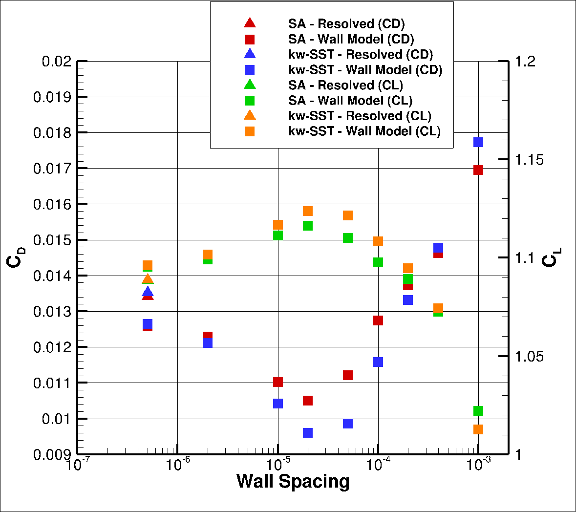
Fig. 5.5.11 Integrated loads values for the NACA0012 case at \(10^o\) for a range of wall spacings for the Spalart-Allmaras and \(k-\omega\) SST turbulence models.#
At a higher angle of attack of \(10^o\), the differences between the wall-resolved and wall-model simulations are reduced. At low wall spacings excellent agreement is seen between wall-resolved and wall-model simulations. The best agreement is once again seen at wall spacings of 0.0001 and 0.0002, where the error on the lift and drag coefficients is under 1% and 5% respectively for the Spalart-Allmaras turbulence model. Once again the the Spalart-Allmaras turbulence wall model simulations seem to perform better than the \(k-\omega\) SST wall model predictions. The integrated loads at the highest examined angle of attack of \(15^o\) are shown in Table 5.5.4 and Fig. 5.5.12.
Wall Spacing |
CL (Spalart-Allmaras) |
CL (\(k-\omega\) SST) |
CD (Spalart-Allmaras) |
CD (\(k-\omega\) SST) |
|---|---|---|---|---|
5E-07 (resolved) |
1.5297564 |
1.5185145 |
0.0251760 |
0.0260543 |
5E-07 |
1.5492167 |
1.5408299 |
0.0231829 |
0.0238758 |
2E-06 |
1.5628159 |
1.5627701 |
0.0221807 |
0.0221119 |
1E-05 |
1.5935174 |
1.6096414 |
0.0192190 |
0.0176531 |
2E-05 |
1.5974993 |
1.6213546 |
0.0188605 |
0.0164618 |
5E-05 |
1.5631734 |
1.5867074 |
0.0222658 |
0.0198286 |
0.0001 |
1.5170764 |
1.4840374 |
0.0274184 |
0.0306383 |
0.0002 |
0.7113100 |
0.7217588 |
0.1765999 |
0.1793623 |
0.0004 |
0.7508150 |
0.7638725 |
0.1655428 |
0.1669165 |
0.001 |
0.9306330 |
0.8796866 |
0.1159778 |
0.1310237 |
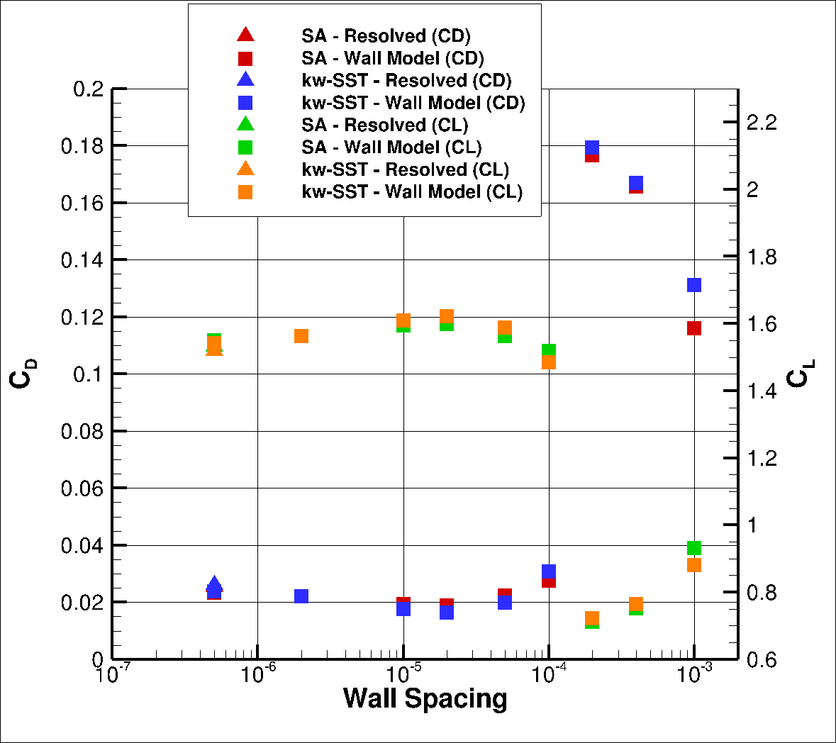
Fig. 5.5.12 Integrated loads values for the NACA0012 case at \(15^o\) for a range of wall spacings for the Spalart-Allmaras and \(k-\omega\) SST turbulence models.#
At the highest angle of attack of \(15^o\), which is close to the maximum lift coefficient, the wall model simulations perform poorer than at lower angles of attack. Reasonable agreement is obtained at low wall spacings up to 0.0001, however, the agreement worsens significantly at wall spacings of 0.0002 and 0.0004. This condition has a significant pressure gradient, and currently pressure gradient effects are not included in the wall model. Hence, when significant pressure gradients are expected, the wall spacing will be limited when using the wall model. The predictions are analysed further by analysing the surface pressure predictions shown in Fig. 5.5.13.
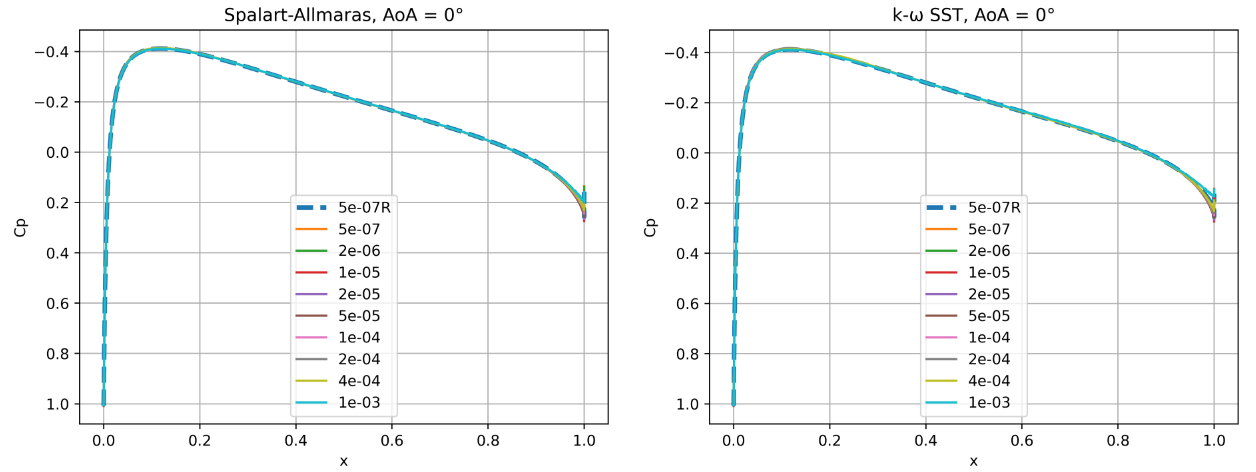
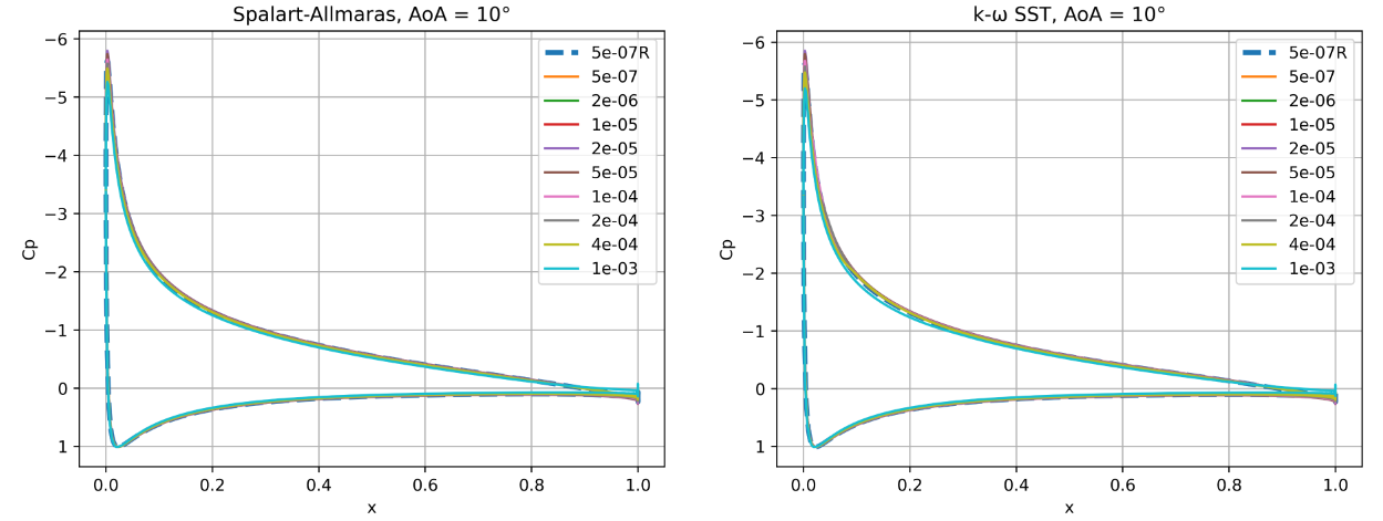
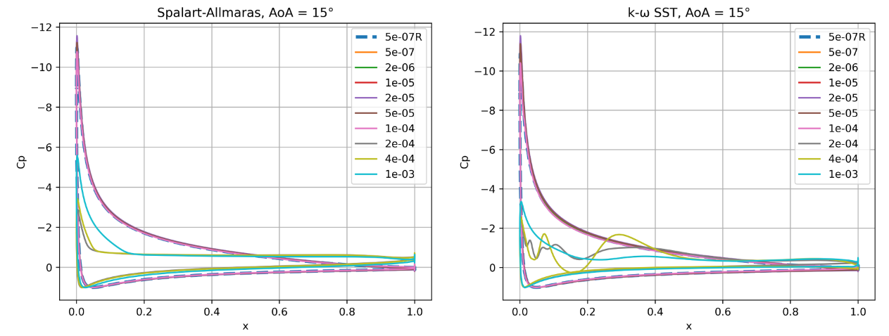
Fig. 5.5.13 Surface pressure coefficient predictions for the NACA0012 case for wall-resolved (R) and wall-model simulations at three angles of attack for the Spalart-Allmaras and \(k-\omega\) SST turbulence models.#
At an angle of attack of \(0^o\), the surface pressure coefficient predictions are close to identical across all wall spacings, with minor differences seen near the trailing edge of the airfoil. As the angle of attack increases to \(10^o\), the suction peak also reduces as the wall spacing is increased, with an increasing error for the highest wall spacings. This behaviour is similar for both Spalart-Allmaras and \(k-\omega\) SST turbulence models. At the highest examined angle of attack of \(15^o\), for the three highest wall spacings, the suction peak is significantly reduced with the pressure no longer recovering at the trailing edge, indicating significant separation over the airfoil. The curves appear to be smoother for the Spalart-Allmaras turbulence model with some noise in the \(k-\omega\) SST pressure curves. At lower wall spacings, the suction peak is reduced slightly compared to the resolved simulation, but the agreement is reasonable. The skin friction distributions are also extracted, shown in Fig. 5.5.14.
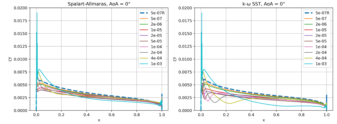
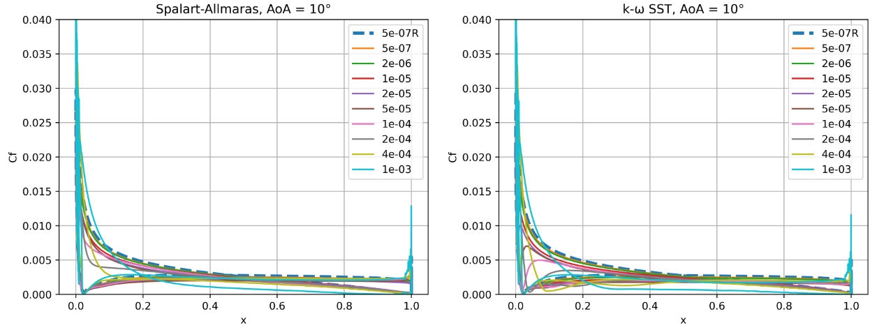
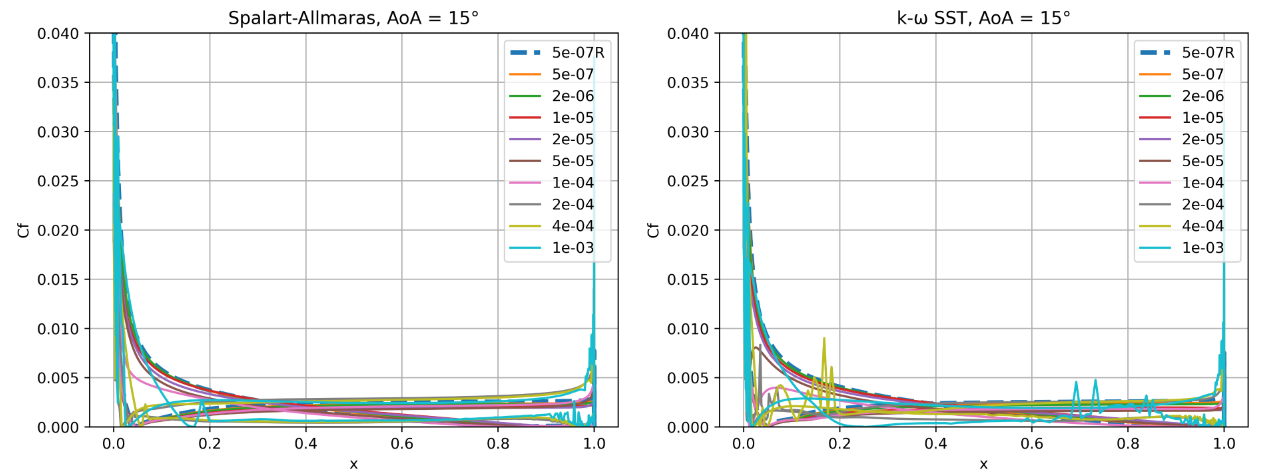
Fig. 5.5.14 Skin friction coefficient predictions for the NACA0012 case for wall-resolved (R) and wall-model simulations at three angles of attack for the Spalart-Allmaras and \(k-\omega\) SST turbulence models.#
The skin friction coefficient curves indicate greater differences between the two turbulence models. At an angle of attack of \(0^o\), very good agreement with the resolved simulation is obtained for the Spalart-Allmaras turbulence model for most wall spacings with a slightly lower skin friction magnitude along the chord of the airfoil. For the three highest wall spacings, the shape of the curve changes slightly with a much higher second skin friction peak. For the \(k-\omega\) SST turbulence model, the skin friction curves, highlight a deeper valley for most wall spacings, indicating that the flow is laminar for a number of wall spacings near the leading edge. This is likely the main cause behind the larger error on the drag values when compared to the Spalart-Allmaras wall model predictions. As the angle of attack is increased to \(10^o\) the skin friction predictions improve with generally good agreement with the resolved simulation across a wide range of wall-spacings, although at the higher range of wall spacings, the peak skin friction on the upper surface seems to be underpredicted. At the highest angle of attack, good behaviour is seen for the low wall spacings, however, for the highest three wall spacing curves, the skin friction goes to zero, very early along the chordwise direction. Significant oscillations can also be observed in the \(k-\omega\) SST results. To examine the validity of the wall model further for the NACA0012 airfoil, we extract the velocity profiles at two chordwise locations of x/c=0.3 and 0.8 across the three angles of attack and two turbulence models, shown in Fig. 5.5.15.
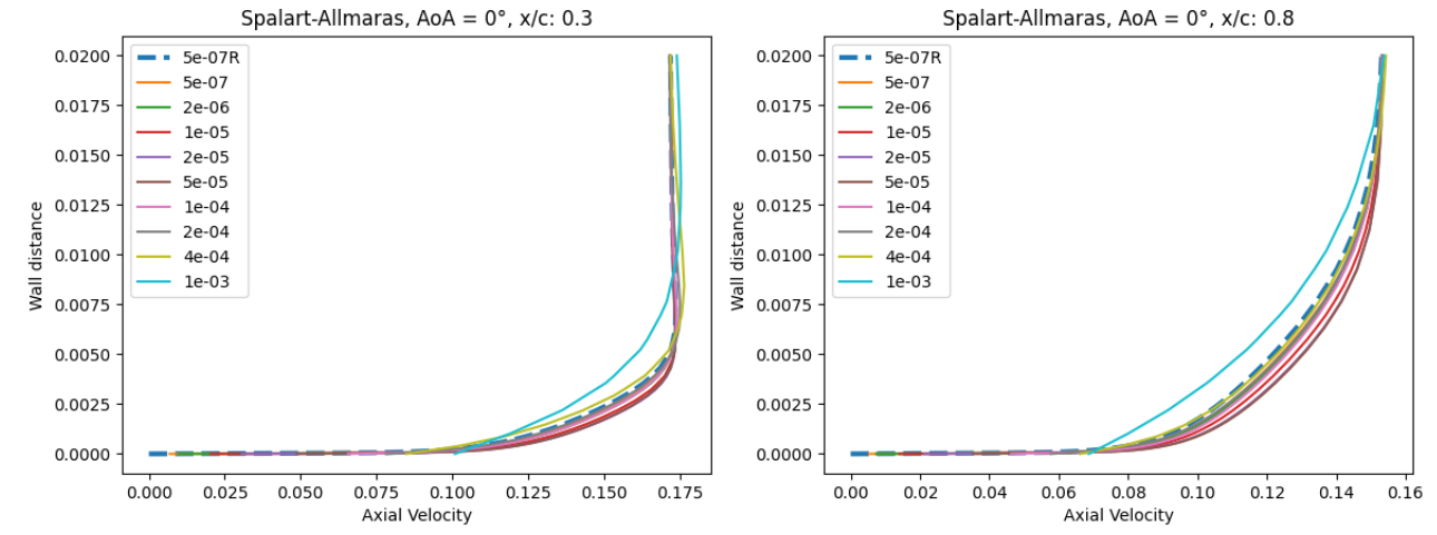
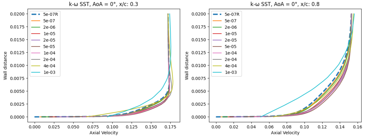
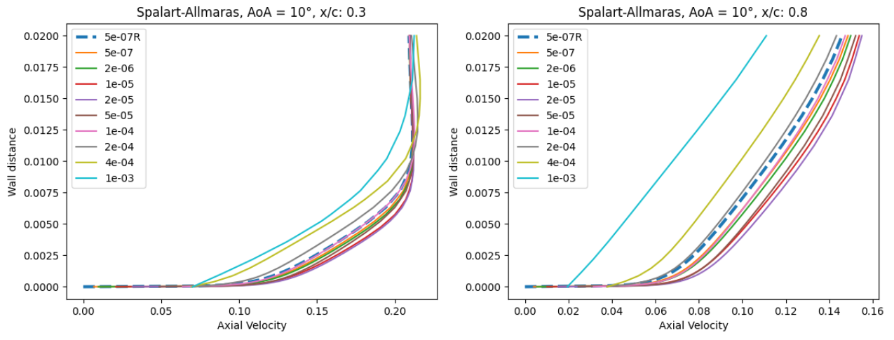
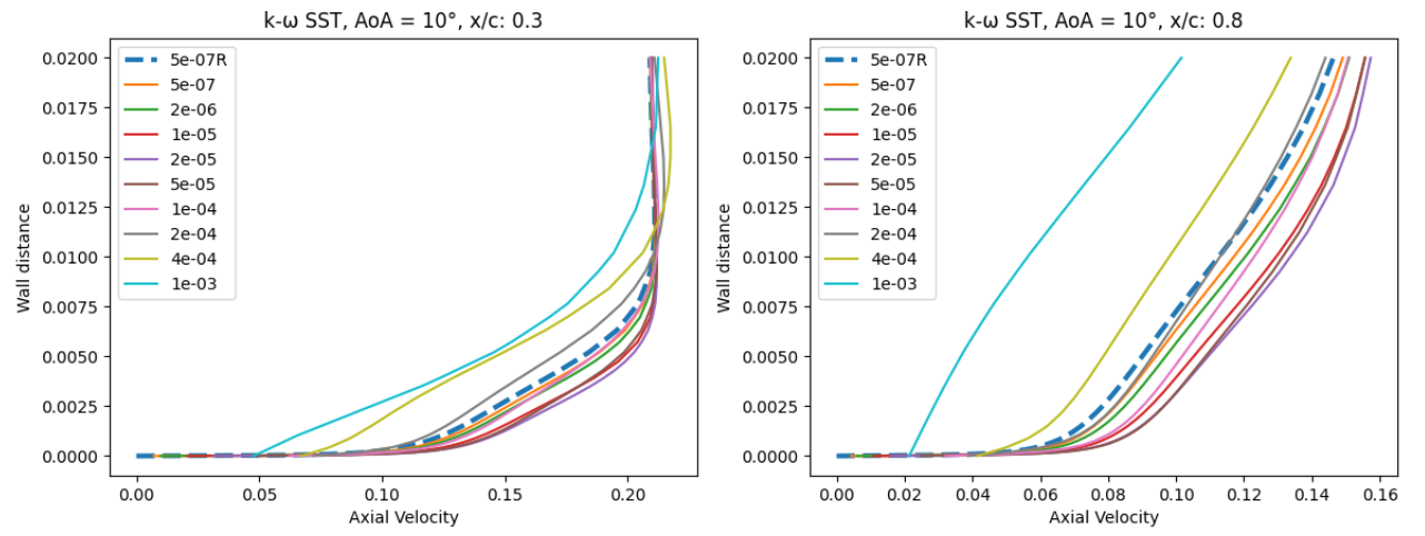
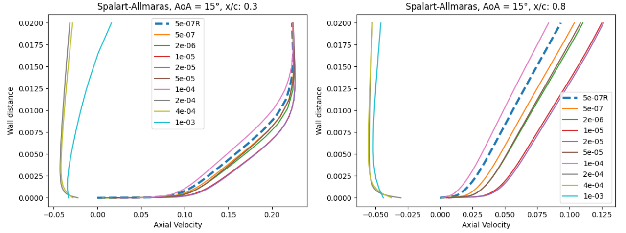
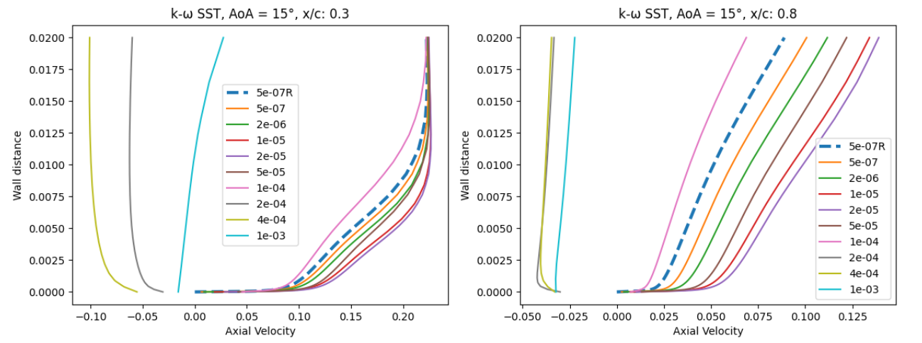
Fig. 5.5.15 Velocity profile predictions for the NACA0012 case for wall-resolved (R) and wall-model simulations at three angles of attack and two chordwise locations for the Spalart-Allmaras and \(k-\omega\) SST turbulence models.#
At an angle of attack of \(0^o\) excellent agreement is obtained for most wall spacings for the axial velocity profiles at both chordwise locations with the resolved simulation. For the Spalart-Allmaras turbulence model, the highest wall spacing velocity profile deviates from the others in the shape. For the \(k-\omega\) SST turbulence model an even larger error on the velocity profile is observed with lower axial velocities observed across the boundary layer than for the resolved simulation. The 4e-04 also shows a minor error at x/c=0.3 with a lower axial velocity close to the wall and higher velocity magnitude outside the boundary layer. At a higher angle of attack of \(10^o\), larger differences are observed between the wall-resolved and wall-model simulations. For both turbulence models, the velocity profiles are fairly reasonable for most wall spacings at x/c=0.3. At x/c=0.8 the two highest wall spacing see significant deviations from the resolved simulations, with much lower axial velocity across the boundary layer. At \(15^o\) the velocity profiles for wall spacings of 1e-03, 4e-04 and 2e-04 are no longer physical as the flow is completely separated as indicated by the negative axial velocity. The agreement for the other wall spacings with the resolved simulation is reasonable for both turbulence models. To examine why such high differences were observed in the pressure and skin friction coefficients as well as the velocity profiles at the highest angle of attack, the flowfield streamlines were extracted from the wall-resolved and wall-model (\(y^+\) ~100) solutions shown in Fig. 5.5.16.
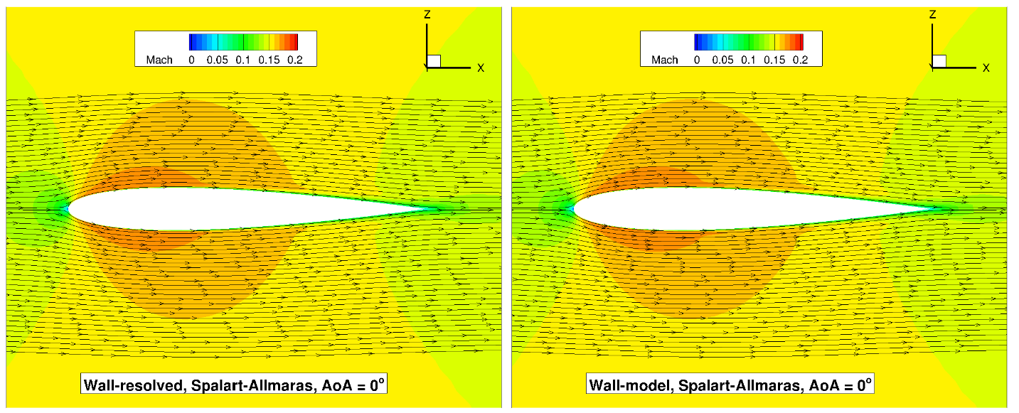
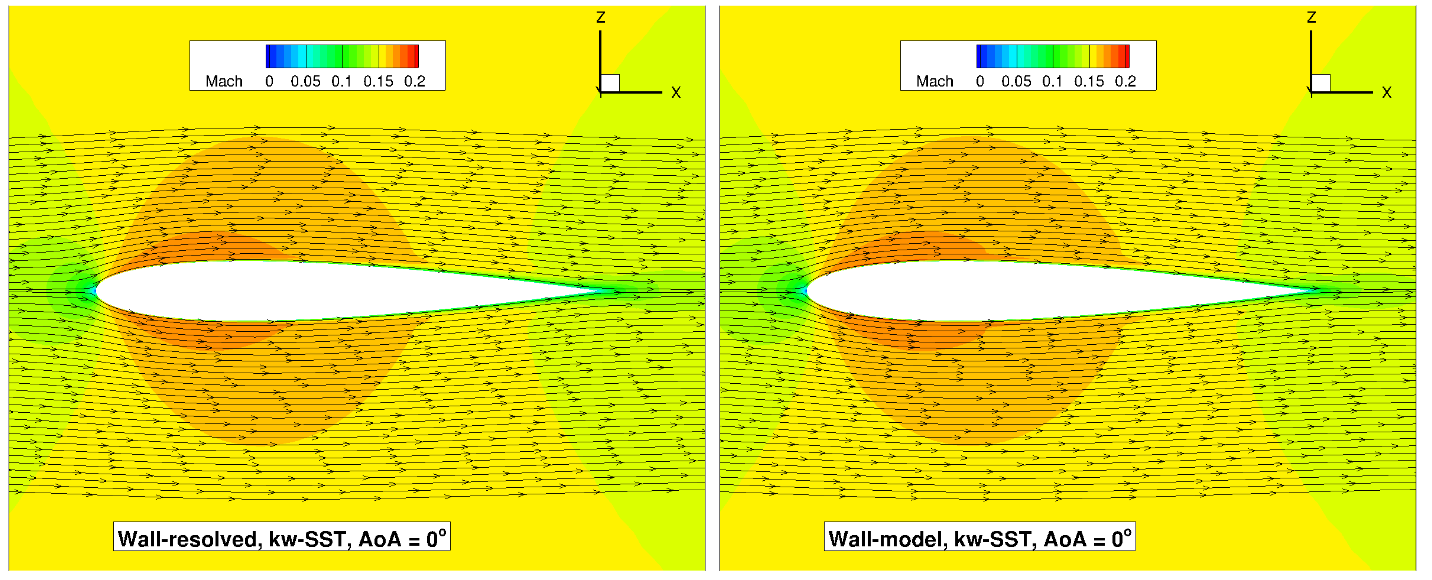
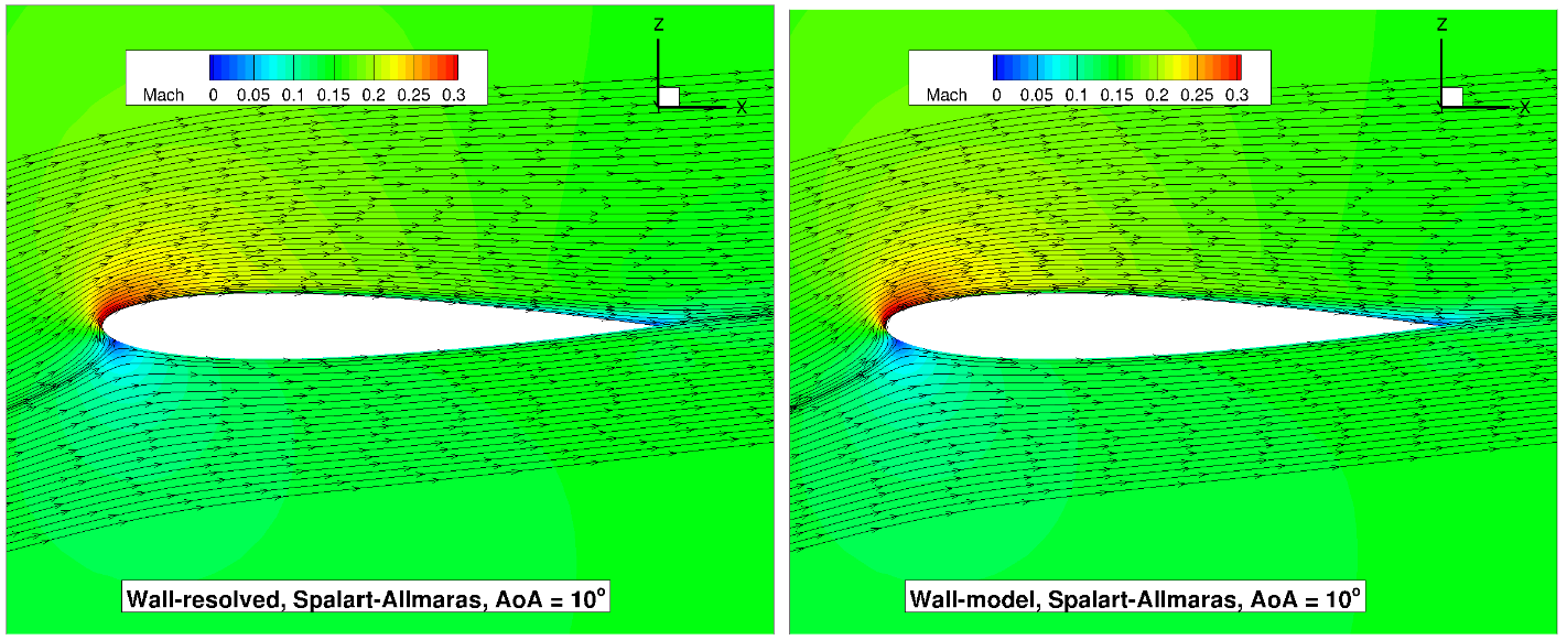
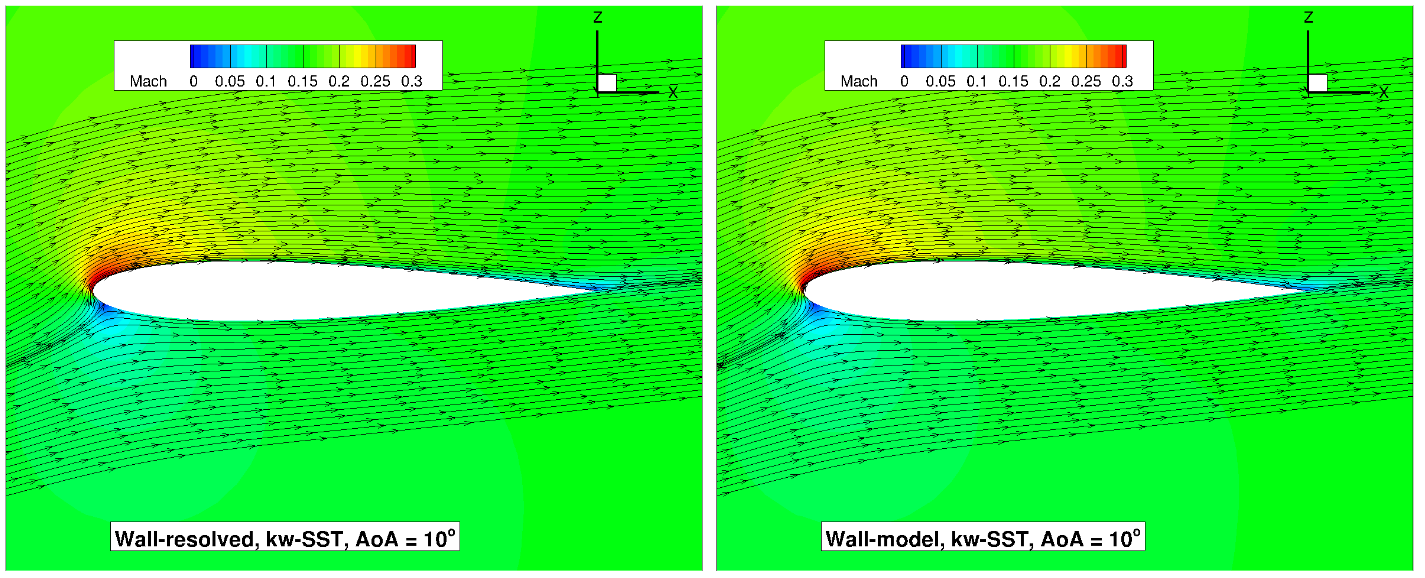
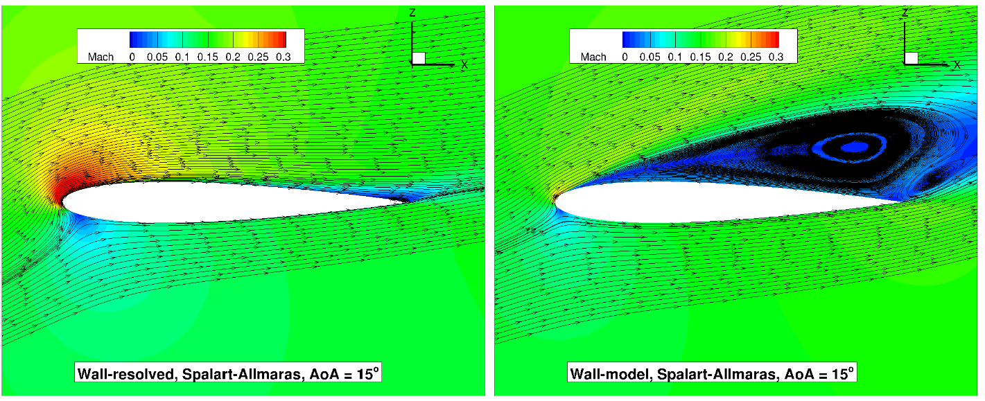
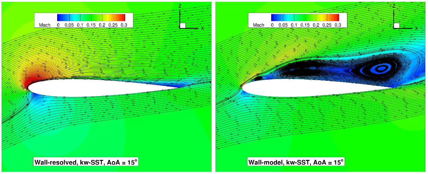
Fig. 5.5.16 Volume streamlines for the NACA0012 case for wall-resolved (R) and wall-model (at ~100 \(y+\)) simulations at three angles of attack for the Spalart-Allmaras and \(k-\omega\) SST turbulence models.#
The flowfield streamlines show a very similar flowfield at \(0^o\) angle of attack for both wall-resolved and wall-model simulations for both turbulence models. The flow is highly symmetrical with a minor acceleration over the leading edge. As the angle of attack is increased to \(10^o\), qualitatively, once again the flowfields show a high degree of consistency. The acceleration is now much sharper with flow near the trailing edge going towards zero Mach number. This indicates the onset of trailing edge separation. At the highest angle of attack of \(15^o\), the wall-model results no longer resemble the wall-resolved simulations. The wall-resolved simulations predict a small pocket of separated flow near the trailing edge, whereas the wall-model simulation lead to a completely stalled flow over the majority of the airfoil chord. The nature of the stalled flow is also slightly different for both turbulence models, with the Spalart-Allmaras simulation leading to a large recirculation bubble, with the \(k-\omega\) SST model predicting multiple smaller recirculations. This case highlights the inability of the current wall model to predict the flowfield and integrated loads under strong pressure gradients. The wall model, however behaved very well at the two lower examined angles of attack of \(0^o\) and \(10^o\).
ONERAM6 Wing Case#
Simulation Setup#
The next case under consideration is the ONERAM6 wing case in transonic conditions. This case aims to evaluate the wall model for a 3D configuration in the presence of a shock-induced separation and strong pressure gradients. The ONERAM6 wing case is a standard CFD validation case for transonic flows, with the results from wall-resolved simulations using Flow360 available in the ONERAM6 wing case study. The flow conditions under consideration are a Mach number of 0.84, Reynolds number based on MAC of 11.72 million at an angle of attack of 3.06 degrees. The grids were generated using our automated meshing workflow. The surface grid for this case is shown in Fig. 5.5.17.
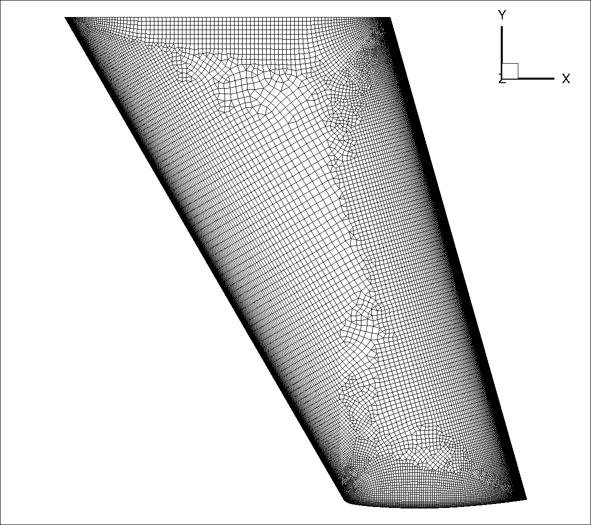
Fig. 5.5.17 ONERAM6 wing surface grid used for the wall-resolved and wall-model simulations.#
The surface grid is fixed for both wall-resolved and wall-model simulations. The surface grid has 86,280 nodes. Anisotropic layers are grown from the the leading and trailing edges, to resolve the areas of the flow with strong flow gradients, although no attempt is made to refine the mesh near the shock. A set of volume grids were generated with spacing values ranging from 5e-07 to 1e-03, leading to grids ranging from 15.3 million nodes to 2.3 million nodes. A slice through the volume at the wing mid-span of the wall-resolved grid and wall model grid with a wall spacing of 2e-04 (approximately \(y^+\) ~100 is shown in Fig. 5.5.18.
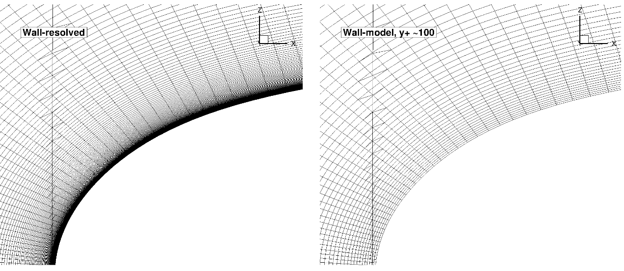
Fig. 5.5.18 Comparison of the wall-resolved (top) and wall-model (\(y^+\) ~100 (bottom) volume grids for the ONERAM6 wing case.#
Similarly to the NACA0012 airfoil, from this view, the wall-model and wall-resolved grids look very similar, although the wall model grid has fewer anisotropic layers leading to a reduction in node counts from 15.3 million to 4.8 million. The simulations were performed using both the Spalart-Allmaras and \(k-\omega\) SST turbulence models. The CFL number was ramped up from 1 to 200 over 5000 pseudo-steps with a total number of pseudo-steps equal to 10000, even though in many cases, fewer pseudo-steps could have been used. Convergence was excellent for most cases, although it was not obtained for the highest wall spacing of 1e-03 when using the \(k-\omega\) SST turbulence model. This is due to the fact that the \(y^+\) value is around 1000 over the main portion of the wing and jumps to an unphysical value of 10000 in the separated region (shock-induced separation), during the convergence of the simulation.
Numerical Results#
Firstly, the integrated loads are compared for wall-resolved and wall-model simulations for both examined turbulence models, shown in Table 5.5.5. The same data is shown in graphical format in Fig. 5.5.19
Wall Spacing |
CL (Spalart-Allmaras) |
CL (\(k-\omega\) SST) |
CD (Spalart-Allmaras) |
CD (\(k-\omega\) SST) |
|---|---|---|---|---|
5E-07 (resolved) |
0.2745839 |
0.2709627 |
0.0174882 |
0.0173155 |
5E-07 |
0.2750711 |
0.2716485 |
0.0172173 |
0.0170549 |
2E-06 |
0.2753277 |
0.2724487 |
0.0170231 |
0.0167591 |
1E-05 |
0.2765591 |
0.2750969 |
0.0162665 |
0.0158812 |
2E-05 |
0.2771044 |
0.2761809 |
0.0160069 |
0.0155393 |
5E-05 |
0.2744205 |
0.2733292 |
0.0170425 |
0.0162485 |
0.0001 |
0.2727455 |
0.2711933 |
0.0173144 |
0.0166847 |
0.0002 |
0.2726556 |
0.2689671 |
0.0172488 |
0.0171784 |
0.0004 |
0.2718576 |
0.2657272 |
0.0171138 |
0.0175339 |
0.001 |
0.2701289 |
0.0171885 |
||
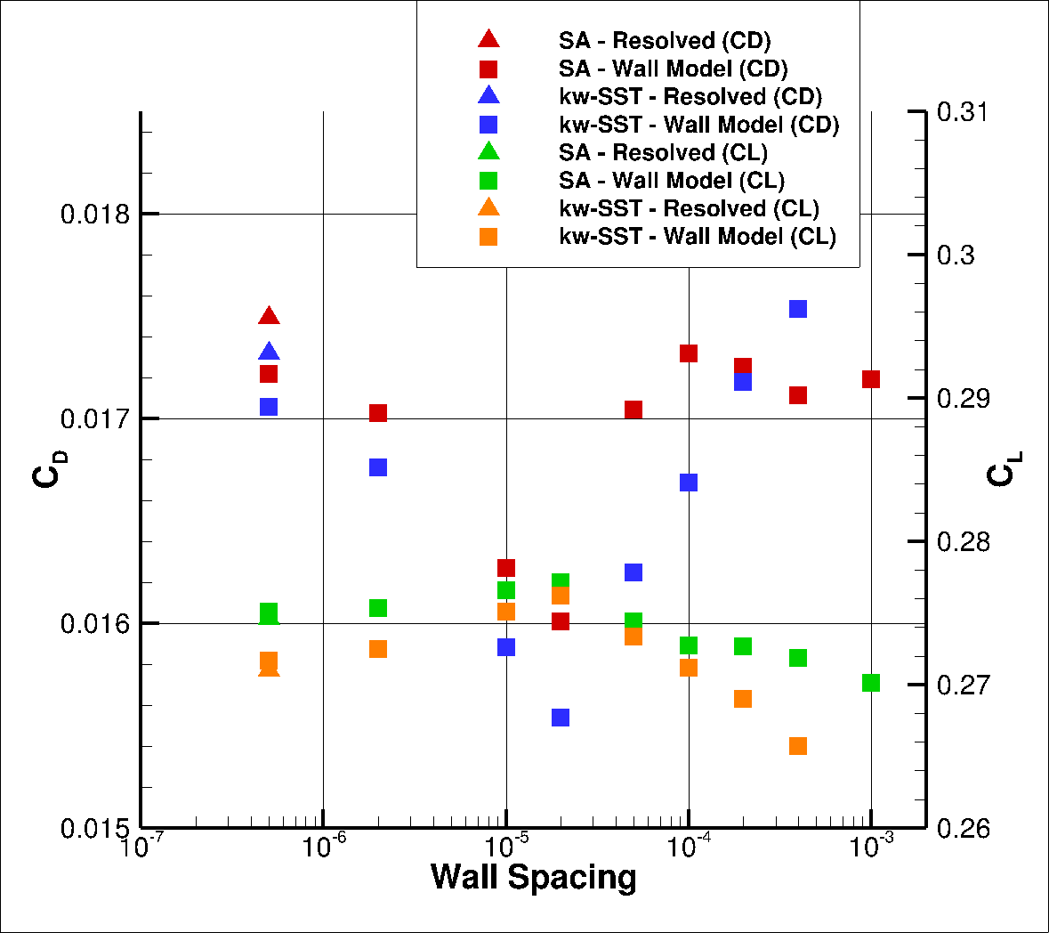
Fig. 5.5.19 Integrated loads values for the ONERAM6 case for a range of wall spacings for the Spalart-Allmaras and \(k-\omega\) SST turbulence models.#
The wall model simulations for this case show excellent agreement with wall-resolved simulations, across the examined wall spacings. Similarly as for the NACA0012 airfoil cases, at low wall spacings the agreement is quite close and reduces as the spacing is increased in both lift and drag, with the lift being slightly overpredicted and drag being slightly underpredicted. The agreement significantly improves at wall spacings of 5e-05 to 0.0004. For a wall spacing of 2e-04, the lift and drag predictions are within 1% of the wall resolved simulations for both turbulence models. To examine this in greater detail, the \(y^+\), are extracted at two spanwise locations, near the mid-span (0.44) and near the tip of the wing (0.9), shown in Fig. 5.5.20.
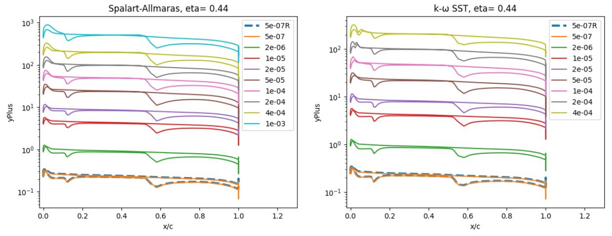
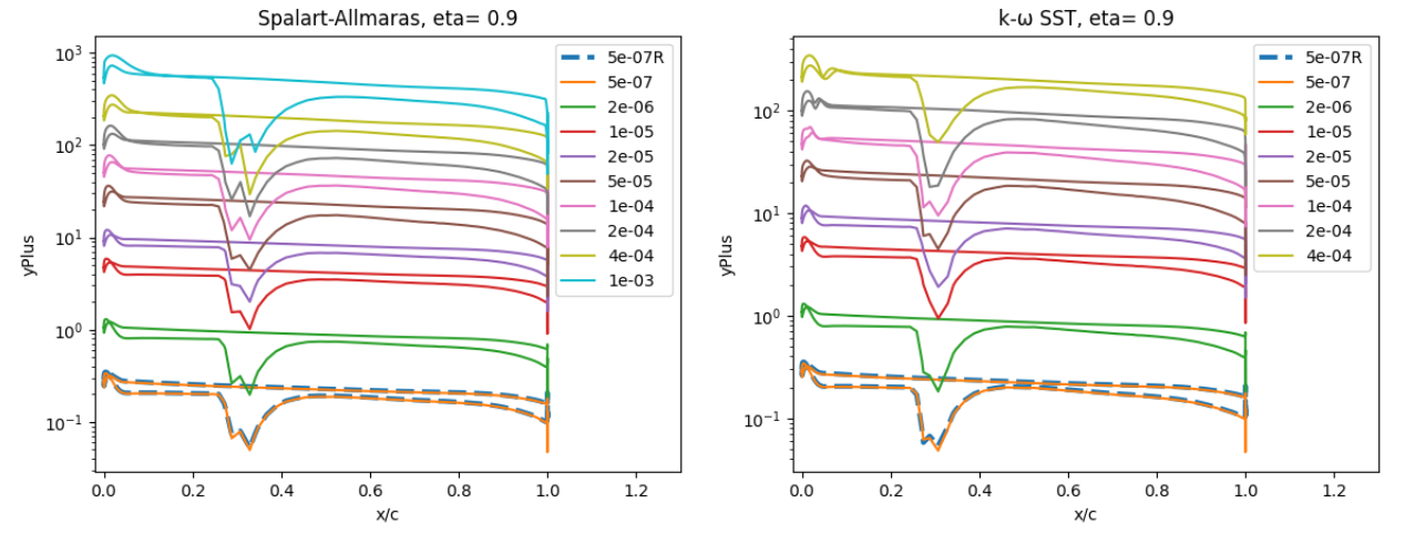
Fig. 5.5.20 Y+ values along the ONERAM6 wing for wall-resolved (R) and wall-model simulations at two spanwise locations for the Spalart-Allmaras and \(k-\omega\) SST turbulence models.#
The \(y^+\) curves show the presence of two valleys at the inboard spanwise location and a single valley of a higher magnitude at the spanwise location near the wing tip, which are associated with the presence of shocks. The wall spacings with the best agreement in integrated loads once again correspond to \(y^+\) values of 50 to 100, although here very good agreement was also obtained at a \(y^+\) of 200. The poorest agreement is obtained in the buffer region and at very high \(y^+\) values. The surface pressure predictions are analysed next, shown in Fig. 5.5.21.
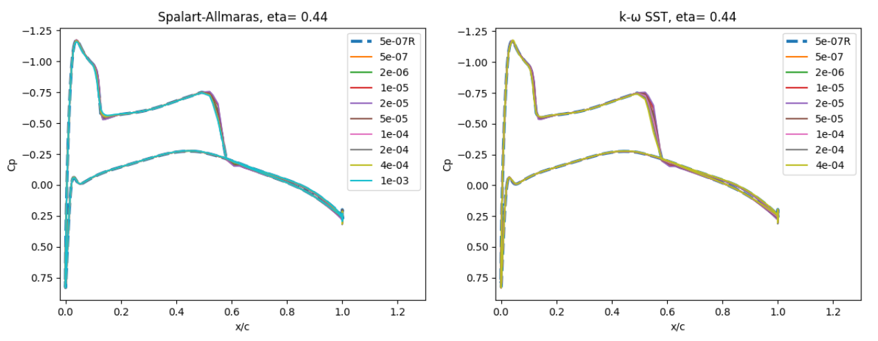
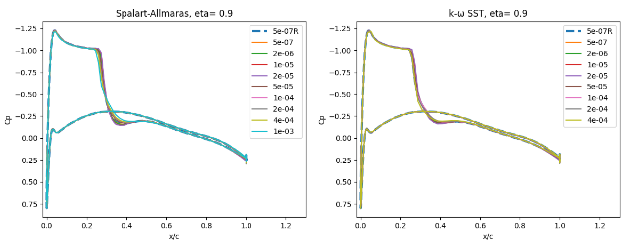
Fig. 5.5.21 Surface pressure coefficient predictions for the ONERAM6 wing case for wall-resolved (R) and wall-model simulations at two spanwise locations for the Spalart-Allmaras and \(k-\omega\) SST turbulence models.#
The surface pressure predictions at the two spanwise locations, show a very low sensitivity to wall spacing. At eta=0.44 two shocks are present along the chordwise direction, whereas at eta=0.9 a single strong shock is located at approximately x/c=0.3. The use of the wall model appears to have a minor impact on the shock locations, but also leads to a poorer resolution of the shock at high wall spacing. The skin friction predictions are shown in Fig. 5.5.22.
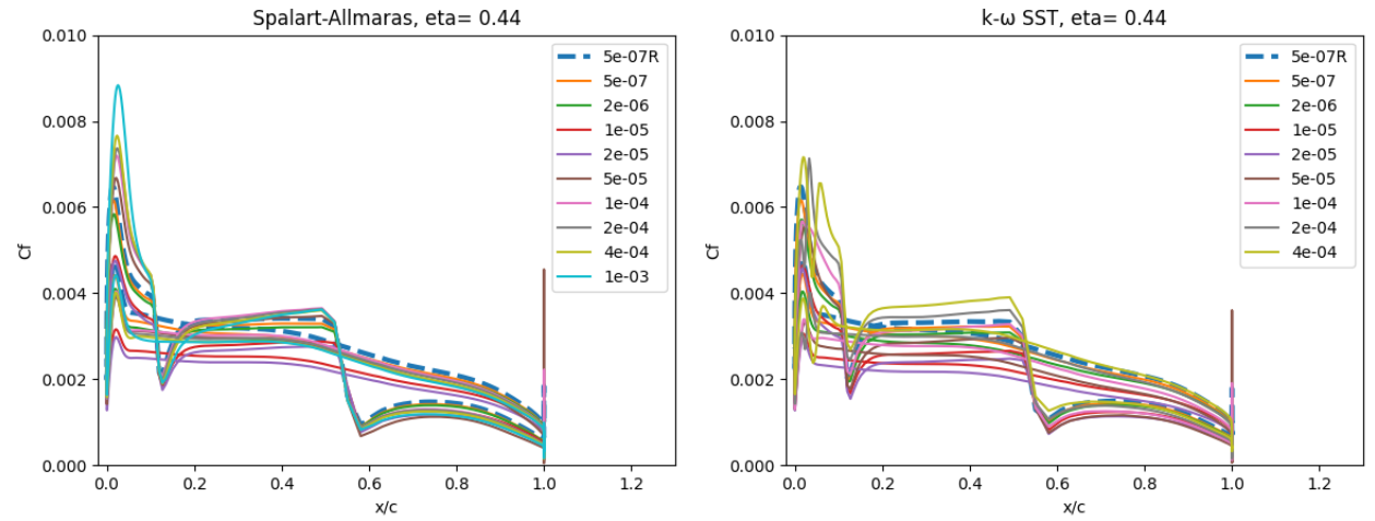
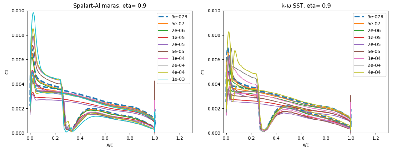
Fig. 5.5.22 Skin friction coefficient predictions for the ONERAM6 wing case for wall-resolved (R) and wall-model simulations at two spanwise locations for the Spalart-Allmaras and \(k-\omega\) SST turbulence models.#
A slightly higher sensitivity is seen for the surface skin friction. At eta=0.44, the skin friction is underpredicted at low wall spacings and overpredicted at high wall spacings, which is especially visible ahead of the first shock as the flow accelerates over the leading edge of the wing section. The general skin friction distribution trend, however, is captured well across all wall spacings. Similar observations can be made at the section near the wing tip. The Spalart-Allmaras and \(k-\omega\) SST turbulence model also appear to behave differently near the pressure suction peak in terms of the skin friction curve, as a highly non-linear behaviour is seen for the \(k-\omega\) SST turbulence model. As this is a 3D geometry, the surface pressure and skin friction distributions are also examined from a qualitative perspective over the entire wing, shown in Fig. 5.5.23-Fig. 5.5.24.
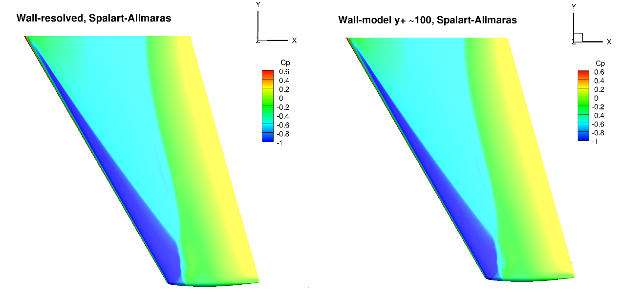
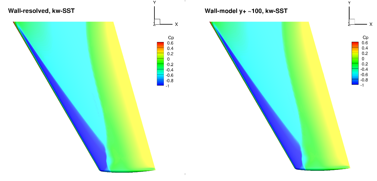
Fig. 5.5.23 Surface pressure coefficient predictions for the ONERAM6 wing case for wall-resolved (R) and wall-model (~100 \(y+\)) simulations for the Spalart-Allmaras and \(k-\omega\) SST turbulence models.#
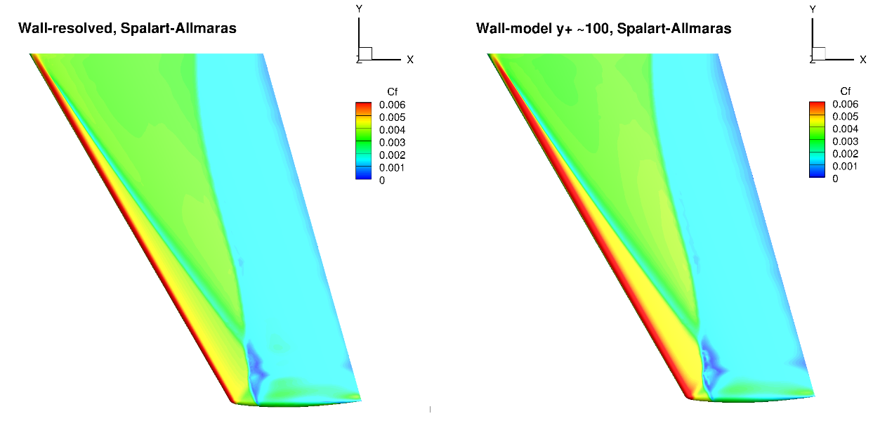
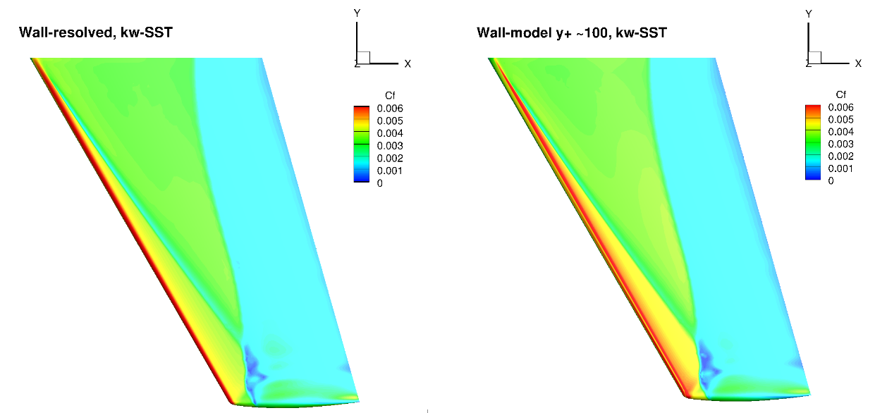
Fig. 5.5.24 Surface skin friction coefficient predictions for the ONERAM6 wing case for wall-resolved (R) and wall-model (~100 \(y+\)) simulations for the Spalart-Allmaras and \(k-\omega\) SST turbulence models.#
The surface pressure distributions across the entire wing show a very high degree of consistency for the wall-resolved and wall-model simulations and both turbulence models. This shows the high quality of the solution coming from the wall model. The skin friction distributions are also very similar with the wall-model simulations predicting a slightly higher skin friction magnitude near the leading edge and over a larger portion of the chord, across the entire wing. There are also minor differences in the shock-induced separation region. To examine these findings further we extracted the velocity profiles at the two spanwise locations (eta=0.44 and 0.9) and two chordwise locations of x/c=0.3 ad 0.8, shown in Fig. 5.5.25.
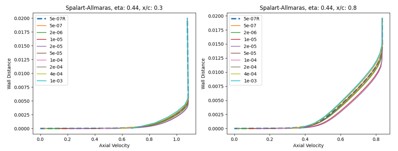
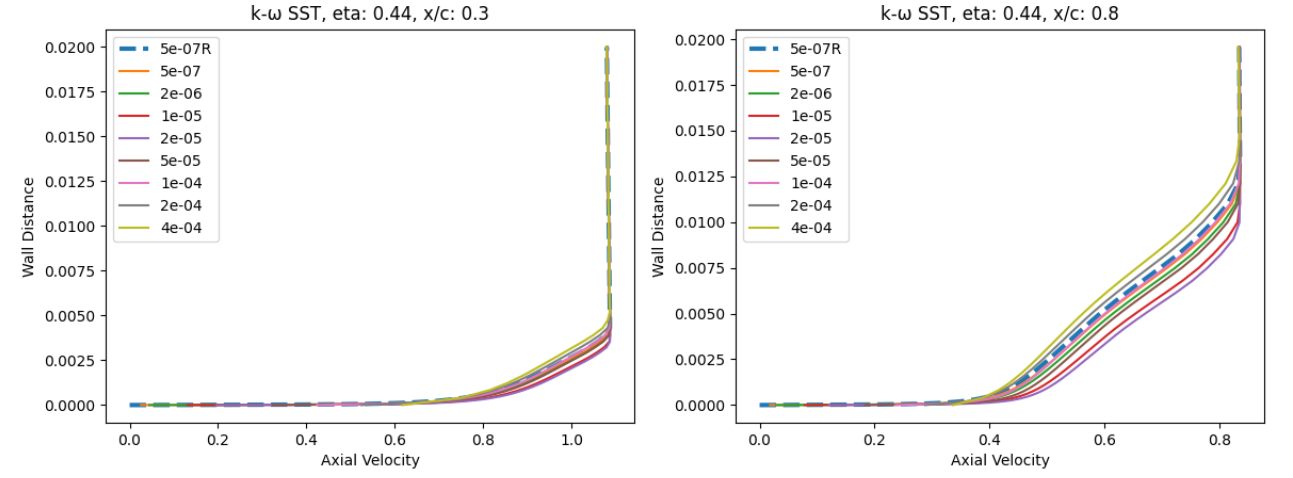
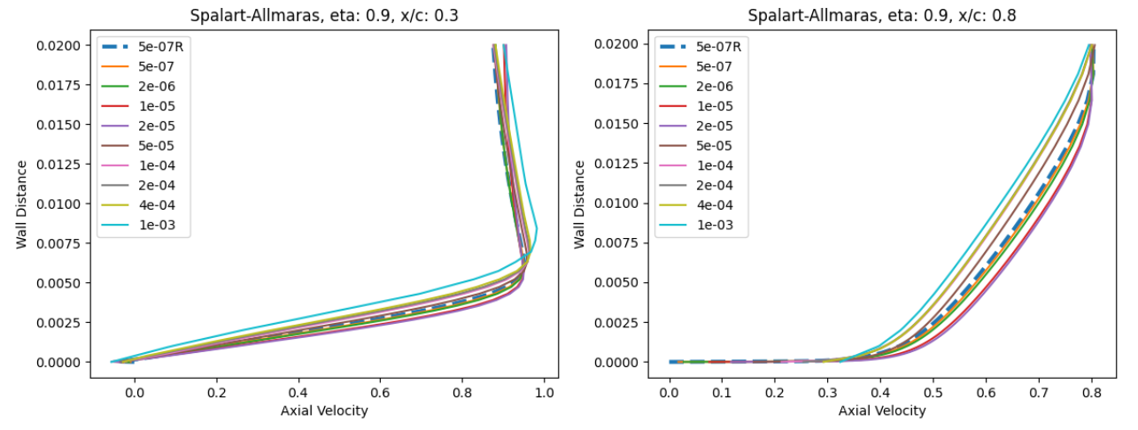
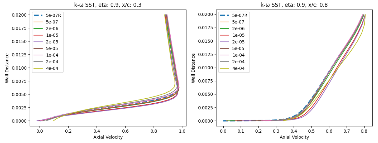
Fig. 5.5.25 Velocity profile predictions for the ONERAM6 wing case for wall-resolved (R) and wall-model simulations at two spanwise and two chordwise locations for the Spalart-Allmaras and \(k-\omega\) SST turbulence models.#
At eta=0.44 and x/c=0.3, the velocity profiles show good agreement across all wall spacings when compared to the wall-resolved simulations, with the largest errors present at wall-spacings of 1e-05 to 2e-05 which are in the buffer region. Further downstream at x/c=0.8 slightly greater differences are observed, especially for the wall spacings in the buffer region, with higher predicted axial velocity magnitudes. The trends are similar for both turbulence models. Further outboard at eta=0.9, similar observations can be made, although the highest wall spacings now also lead to some differences. Here, the highest wall spacing leads to an underprediction of the axial velocity across the boundary layer. A small pocket of separated flow can also be noticed at x/c=0.3 which is well captured by the wall model.
Ahmed Body Case#
Simulation Setup#
The next case under consideration is the Ahmed body case, which is often used as the baseline case for validation in automotive applications, making it a great starting point for wall model validation for automotive cases. The flow conditions under consideration are a Mach number of 0.1728 with a Reynolds number of 4.176 million. The inlet and outlet boundaries are set to farfield with the floor also modeled as a no slip wall or using the wall function approach. The grids were generated by starting from a structured surface grid, and manually generating the volume grids. The surface grid for this case is shown in Fig. 5.5.26.
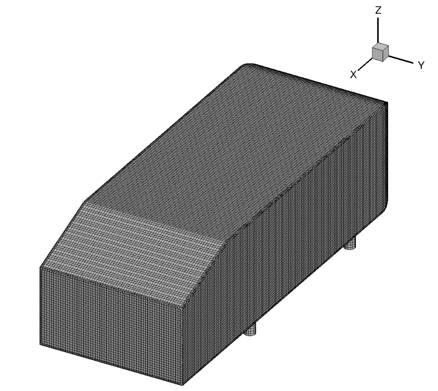
Fig. 5.5.26 Ahmed body surface grid used for the wall-resolved and wall-model simulations.#
The surface grid is fixed for both wall-resolved and wall-model simulations. The surface grid has 39,434 nodes. The spacing is fairly uniform over the entire vehicle. A set of volume grids were generated with spacing values ranging from 5e-07 to 1e-03, leading to grids ranging from 3 million nodes to 0.85 million nodes. A slice through the volume along the centerline of the wall-resolved grid and wall model grid with a wall spacing of 4e-04 (approximately \(y^+\) ~100 is shown in Fig. 5.5.27.
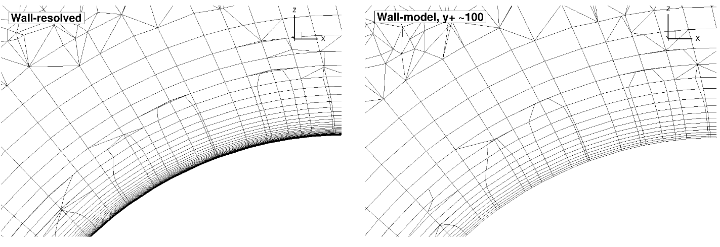
Fig. 5.5.27 Comparison of the wall-resolved (top) and wall-model (\(y^+\) ~100 (bottom) volume grids for the Ahmed body case.#
From this view, the wall-model and wall-resolved grids look very similar, similarly as in the previously examined cases. The wall model grid has fewer anisotropic layers leading to a reduction in node counts from 3 million to 1.1 million. The simulations were performed using both the Spalart-Allmaras and \(k-\omega\) SST turbulence models. The CFL number was ramped up from 1 to 200 over 2000 pseudo-steps with a total number of pseudo-steps equal to 10000, even though in many cases, fewer pseudo-steps could have been used. Tests showed that even higher CFL numbers could have also been used, with the wall model simulations showing slightly better convergence properties with increasing wall spacing.
Numerical Results#
Firstly, the integrated loads are compared for wall-resolved and wall-model simulations for both examined turbulence models, shown in Table 5.5.6. The same data is shown in graphical format in Fig. 5.5.28
Wall Spacing |
CL (Spalart-Allmaras) |
CL (\(k-\omega\) SST) |
CD (Spalart-Allmaras) |
CD (\(k-\omega\) SST) |
|---|---|---|---|---|
5E-07 (resolved) |
0.2838657 |
0.2727445 |
0.3389527 |
0.3246567 |
5E-07 |
0.2833976 |
0.2723599 |
0.3351060 |
0.3203302 |
2E-06 |
0.2815923 |
0.2708006 |
0.3346436 |
0.3197694 |
1E-05 |
0.2817096 |
0.2777542 |
0.3308835 |
0.3120820 |
2E-05 |
0.2789197 |
0.2757056 |
0.3277845 |
0.3087600 |
5E-05 |
0.2772840 |
0.2669671 |
0.3248126 |
0.3031932 |
0.0001 |
0.2811986 |
0.2701703 |
0.3305484 |
0.3151284 |
0.0002 |
0.2895193 |
0.2832801 |
0.3410175 |
0.3253558 |
0.0004 |
0.2936916 |
0.2885895 |
0.3483039 |
0.3300952 |
0.001 |
0.2936290 |
0.3219432 |
0.3620031 |
0.3477800 |
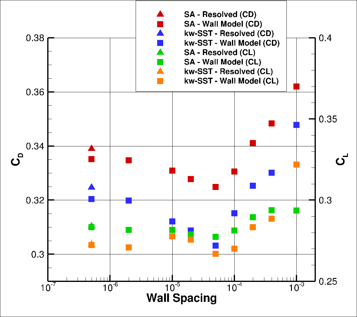
Fig. 5.5.28 Integrated loads values for the Ahmed case for a range of wall spacings for the Spalart-Allmaras and \(k-\omega\) SST turbulence models.#
The integrated loads show excellent agreement for the wall-model simulations when compared to the wall-resolved simulations. At low wall spacings, both the lift and drag coefficients decreases with increasing wall spacing, until a spacing of 5e-05. At a spacing of 0.0001 both the drag and lift start to increase with excellent agreement with the wall-resolved simulations, which slightly worsens at the highest examined wall spacing. The best agreement is seen at a wall spacing of 0.0001 for the Spalart-Allmaras turbulence model and 0.0002 for the \(k-\omega\) SST turbulence model. To examine these differences in greater detail, first the \(y^+\), surface pressure coefficient and skin friction coefficient predictions are extracted along the centerline (y=0), shown in Fig. 5.5.29-Fig. 5.5.31.
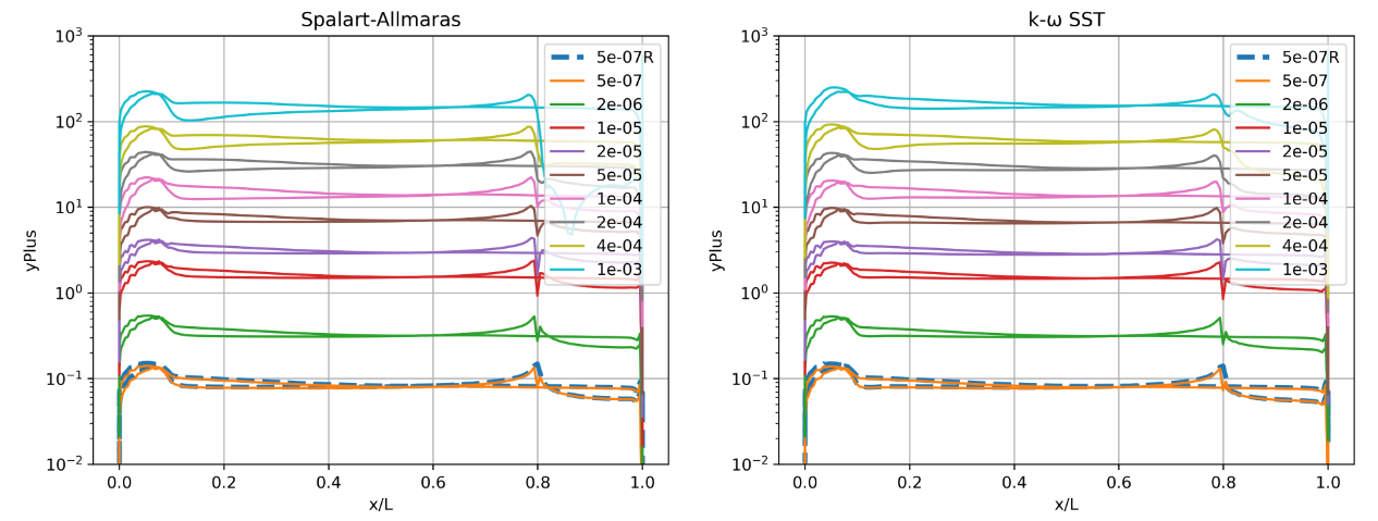
Fig. 5.5.29 Y+ values along the centerline (y=0) of the Ahmed body for wall-resolved (R) and wall-model simulations for the Spalart-Allmaras and \(k-\omega\) SST turbulence models.#
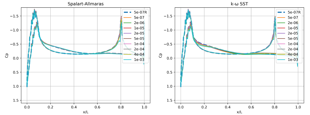
Fig. 5.5.30 Surface pressure predictions along the centerline (y=0) of the Ahmed body for wall-resolved (R) and wall-model simulations for the Spalart-Allmaras and \(k-\omega\) SST turbulence models.#
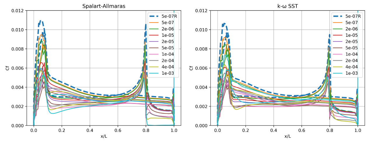
Fig. 5.5.31 Skin friction predictions along the centerline (y=0) of the Ahmed body for wall-resolved (R) and wall-model simulations for the Spalart-Allmaras and \(k-\omega\) SST turbulence models.#
Based on the \(y^+\) distributions, the best integrated loads predictions were obtained at \(y^+\) values of 20 to 50 although the agreement at \(y^+\) of 100 was also very good. A certain degree of non-linearity is present at the front of the car in the \(y^+\) and surface pressure curves, indicating that the curvature of the front of the vehicle is not well-resolved in the mesh. The surface pressure predictions show excellent agreement across all wall spacings with minor differences observed in the second suction peak near the start of the rear ramp, as well as over the car body before the ramp, especially for the \(k-\omega\) SST turbulence model. The skin friction curves, show that for all wall spacings the skin friction magnitude is underpredicted when compared to the wall-resolved simulation, with the differences increasing with increasing wall spacing. This is especially visible in the two skin friction peaks. Here, certain differences are observed past the peaks between the two turbulence models. The Spalart-Allmaras model predicts a deeper skin friction valley as the flow decelerates, with separation present at the highest wall spacing past the rear ramp. Examining these effects further, the velocity profiles were extracted from the solutions at two locations along the centreline corresponding to x/L=0.3 and x/L=0.9. The second point is mid-way down the rear ramp.
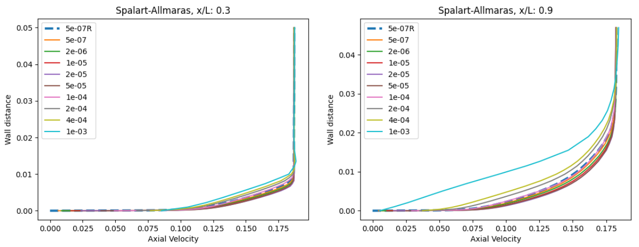
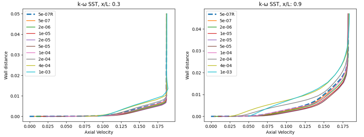
Fig. 5.5.32 Velocity profile predictions for the Ahmed body case for wall-resolved (R) and wall-model simulations at two locations along the centerline (y=0) for the Spalart-Allmaras and \(k-\omega\) SST turbulence models.#
At x/L=0.3, the velocity profiles are consistent for most wall spacings, with the axial velocity slightly decreasing with increasing wall spacing. The differences are slightly higher for the \(k-\omega\) SST turbulence model. At x/L=0.9 on the ramp of the car, greater differences are seen in the velocity profile predictions, especially at higher wall spacings. Flow separation is confirmed for the highest wall spacing when using the Spalart-Allmaras turbulence model as the velocity profile reduces at the first point above the wall. The wall velocity also appears to be different for both examined turbulence models at the highest wall spacing. The agreement is improved at wall spacings of 1e-04 and 2e-04. Finally, the flowfield streamline patterns are extracted from the solutions along the centerline, shown in Fig. 5.5.33.
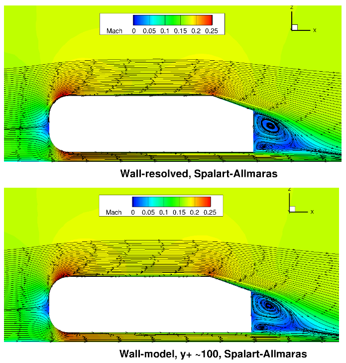
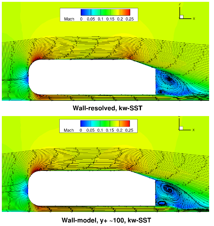
Fig. 5.5.33 Flowfield predictions along the centerline (y=0) for the Ahmed body case for wall-resolved (R) and wall-model (at ~100 \(y+\)) simulations for the Spalart-Allmaras and \(k-\omega\) SST turbulence models.#
Qualitatively, the flowfield streamlines show excellent agreement between wall-resolved and wall-modeled simulations for both examined turbulence models. Although the flow at the back of the car, was not the focus of this study, similar flow features are observed with a larger and smaller recirculation region present. The highly consistent flowfields highlight the applicability of the wall model to automotive applications.
Windsor Body Case#
Simulation Setup#
The final case under consideration is the Windsor body case, which is also aimed at automotive applications. This case was used during the 2nd automotive prediction workshop, and hence is seen as a more realistic automotive test case. The flow conditions under consideration are a Mach number of 0.1175 and Reynolds number of 0.77 million based on the vehicle height. The boundary conditions setup is similar to the Ahmed body case, with the floor modeled as a no slip wall or using wall functions. Only half the vehicle is modeled with a symmetry plane used at the vehicle centerline. The grids were generated using ANSA, with the surface grid shown in Fig. 5.5.34.
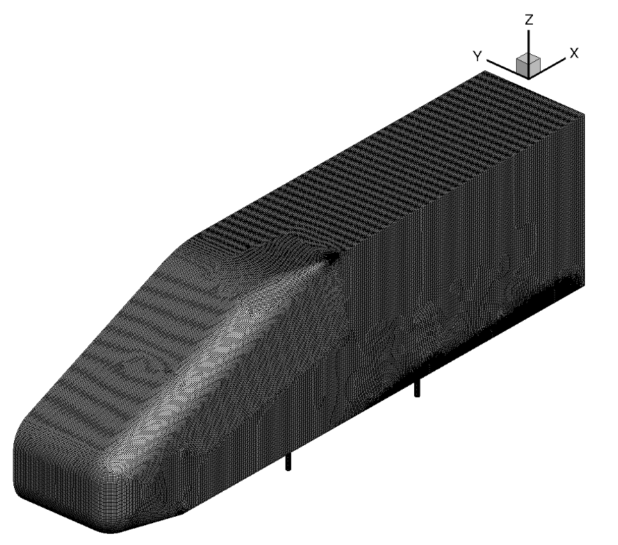
Fig. 5.5.34 Windsor body surface grid used for the wall-resolved and wall-model simulations.#
The surface grid used for both wall-resolved and wall-model simulations is fairly fine and has 152,601 nodes for a half-body. The spacing is fairly uniform over the entire vehicle. A set of volume grids were generated with spacing values ranging from 1e-06 to 2.5e-03, leading to grids ranging from 7.3 million nodes to 2.7 million nodes. The volumetric grid along the symmetry plane for the wall-resolved and wall model grids (spacing of 4e-04, approximately \(y^+\) ~100) is shown in Fig. 5.5.35
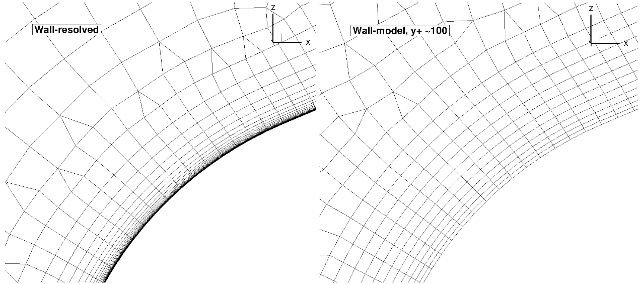
Fig. 5.5.35 Comparison of the wall-resolved (top) and wall-model (\(y^+\) ~100 (bottom) volume grids for the Windsor body case.#
For the Windsor body cases, the number of anisotropic layers was adjusted manually. 25 layers were used for the wall-resolved simulations, which were gradually reduced to 9 layers for the mesh with the highest wall spacing. Here, the differences in the mesh near the wall can be seen clearly, with a prism layers extending deeper into the domain for the wall model grid. For the same height of the anisotropic region, even more layers would need to be used for the wall-resolved mesh. Compared to the automotive prediction workshop grids, no attempt was made at refining the mesh at the rear of the car, as the focus here is on evaluating the wall model rather than direct comparisons with experimental data. The wall model grid shown above, leads to a reduction in node counts from 7.3 million to 3.1 million nodes. The simulations were performed using both the Spalart-Allmaras and \(k-\omega\) SST turbulence models. The CFL number was ramped up from 1 to 200 over 2000 pseudo-steps with a total number of pseudo-steps equal to 10000, even though in many cases, fewer pseudo-steps could have been used. Tests showed that even higher CFL numbers could have also been used, with the wall model simulations showing slightly better convergence properties with increasing wall spacing.
Numerical Results#
Firstly, the integrated loads are compared for wall-resolved and wall-model simulations for both examined turbulence models, shown in Table 5.5.7.
Wall Spacing |
CL (Spalart-Allmaras) |
CL (\(k-\omega\) SST) |
CD (Spalart-Allmaras) |
CD (\(k-\omega\) SST) |
|---|---|---|---|---|
1e-06 (resolved) |
-0.1491836 |
-0.1095171 |
0.3453143 |
0.2940736 |
1e-06 |
-0.1531223 |
-0.1118958 |
0.3424746 |
0.2886777 |
5e-06 |
-0.1558363 |
-0.1216370 |
0.3413276 |
0.2886765 |
2.5e-05 |
-0.1631274 |
-0.1230071 |
0.3389714 |
0.2818219 |
5e-05 |
-0.1688174 |
-0.1260008 |
0.3392483 |
0.2820035 |
1.25e-04 |
-0.1721921 |
-0.1308088 |
0.3427992 |
0.2815498 |
2.5e-04 |
-0.1580500 |
-0.1195373 |
0.3543502 |
0.2915398 |
5e-04 |
-0.1606261 |
-0.1169904 |
0.3637310 |
0.3032360 |
1e-04 |
-0.1716058 |
-0.1234653 |
0.3781859 |
0.3180197 |
2.5e-03 |
-0.1687491 |
-0.1135775 |
0.4028245 |
0.3452181 |
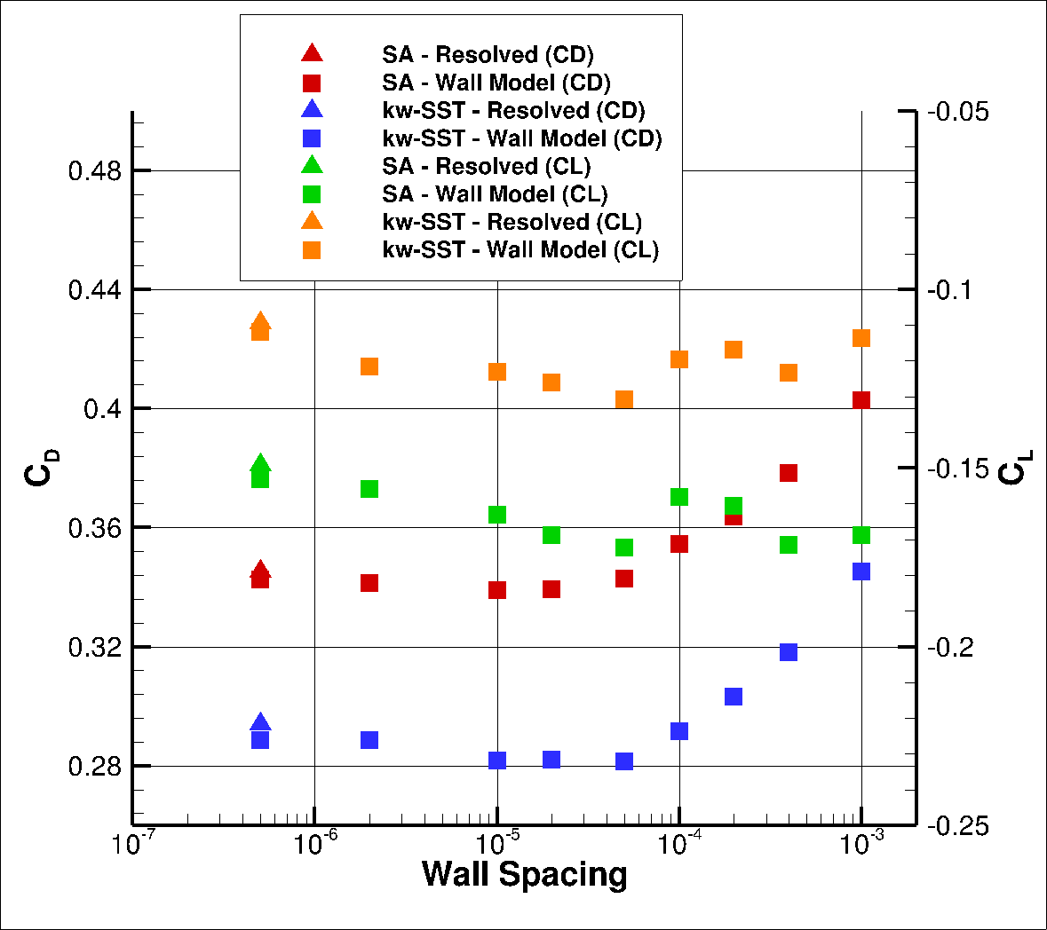
Fig. 5.5.36 Drag values for the Windsor case for a range of wall spacings for the Spalart-Allmaras and \(k-\omega\) SST turbulence models.#
The integrated loads show similar behaviour as for the Ahmed body case. At low wall spacings, both the predicted lift and drag coefficients start to decrease, when compared to wall-resolved simulations up to a wall spacing of 5e-05. As the wall spacing is increased further the lift convergence with wall spacing becomes non-monotonic and the drag increases. For both turbulence models, the best drag prediction agreement is obtained for a wall spacing of 2.5e-04, with the drag values being extremely close to the wall-resolved simulations. To examine these differences in greater detail, first the \(y^+\), surface pressure coefficient and skin friction coefficient predictions are extracted on the symmetry plane, shown in Fig. 5.5.37-Fig. 5.5.39.
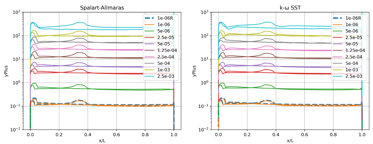
Fig. 5.5.37 Y+ values along the centerline (y=0) of the Windsor body for wall-resolved (R) and wall-model simulations for the Spalart-Allmaras and \(k-\omega\) SST turbulence models.#
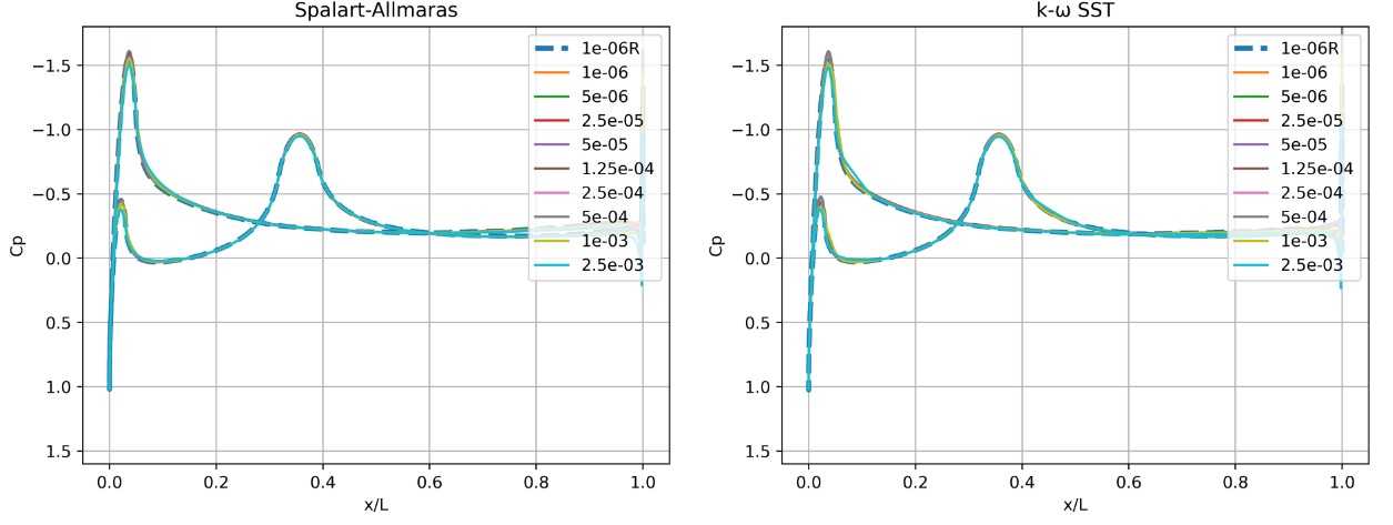
Fig. 5.5.38 Surface pressure predictions along the centerline (y=0) of the Windsor body for wall-resolved (R) and wall-model simulations for the Spalart-Allmaras and \(k-\omega\) SST turbulence models.#
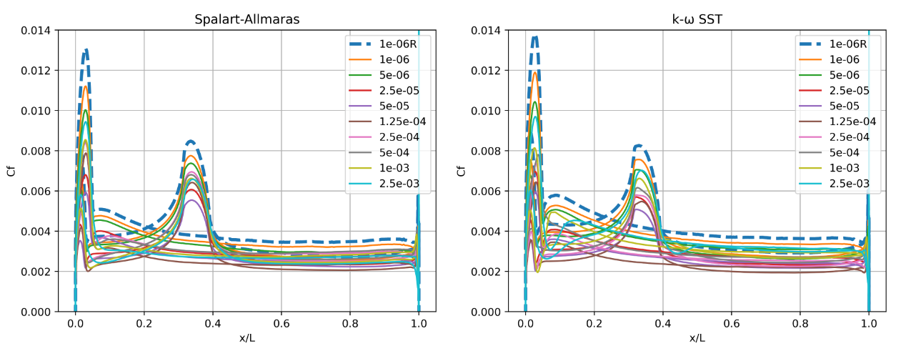
Fig. 5.5.39 Skin friction predictions along the centerline (y=0) of the Windsor body for wall-resolved (R) and wall-model simulations for the Spalart-Allmaras and \(k-\omega\) SST turbulence models.#
The \(y^+\) profiles are consistent between the two turbulence models. Similarly as for the Ahmed body case, the best agreement in integrated loads is obtained for \(y^+\) values of 25-50, although the integrated loads were also reasonable at higher \(y^+\) values. A secondary peak is seen in the \(y^+\) profiles due to the presence of the end of the front ramp. The surface pressure predictions show excellent agreement across all wall spacings, with subtle differences in the suction peak at the front of the car and as the flow separates at the rear of the car. For this case, the pressure curves are consistent between the two turbulence models. The skin friction curves, also generally show reduced peak skin friction as the wall spacing is increased at low wall spacings. The peak skin friction then increases at high wall spacings giving better agreement with the wall-resolved simulation. The trends are captured very well for both turbulence models. Examining these effects further, the velocity profiles were extracted from the solutions at two locations on the symmetry plane corresponding to x/L=0.3 and x/L=0.9.
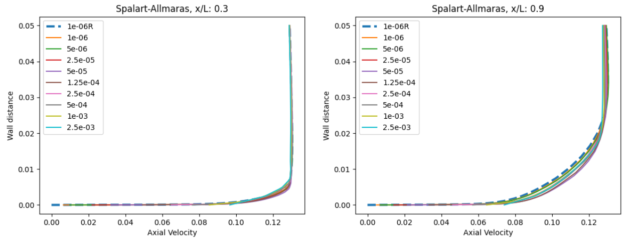
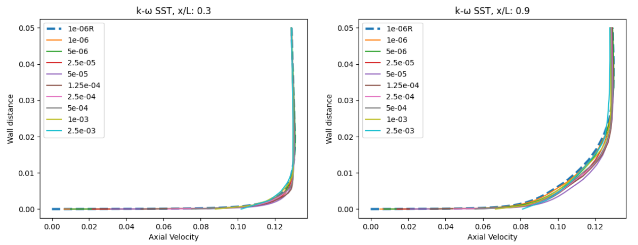
Fig. 5.5.40 Velocity profile predictions for the Windsor body case for wall-resolved (R) and wall-model simulations at two locations along the centerline (y=0) for the Spalart-Allmaras and \(k-\omega\) SST turbulence models.#
The velocity profiles show a high degree of consistency between the wall-resolved and wall-model simulations. The minor differences are slightly larger at x/L=0.9 than at x/L=0.3, however, the excellent agreement across all wall spacings is very promising. There is a minor difference in the wall velocity predicted by the two different turbulent models. Finally, the flowfield streamline patterns are extracted from the solutions on the symmetry plane, shown in Fig. 5.5.41.
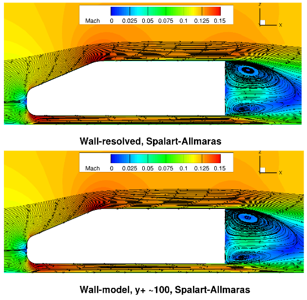
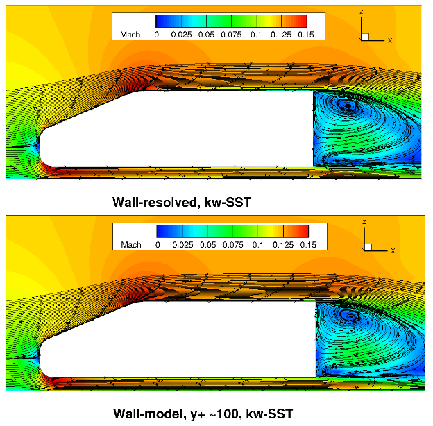
Fig. 5.5.41 Flowfield predictions along the centerline (y=0) for the Windsor body case for wall-resolved (R) and wall-model (at ~100 \(y+\)) simulations for the Spalart-Allmaras and \(k-\omega\) SST turbulence models.#
Similarly as for the Ahmed body case, the flowfields are very consistent between wall-resolved and wall-modelled simulations. The acceleration over the top of the car and between the car underbody and floor is well captured with similar flow patterns in the car wake. Here, slightly different recirculation patterns are predicted when comparing the Spalart-Allmaras and \(k-\omega\) SST turbulence model results. The \(k-\omega\) SST turbulence model predicts a smaller second recirculation eye, which is closer to the floor.
Conclusions#
This case study leads to the following recommendations and conclusions for investigations that include wall modeling:
The wall model has been validated against wall-resolved simulations for a number of test cases including aerospace and automotive applications, leading to very good agreement in the integrated loads predictions.
No robustness issues were found with the wall model even at very high CFL numbers, higher than would be typically used for wall-resolved simulations, although the model robustness will reduce at very high \(y^+\) values of above 1000.
The best agreement in integrated loads was obtained for \(y^+\) values ranging from 1 to 5 and 25 to 100 when compared to wall-resolved simulations. Poorer agreement is obtained when the first layer height is in the buffer region.
The use of the wall model typically has minor impact on the surface pressure prediction, but will lead to an error on the skin friction distributions. Generally, however, the skin friction trends are well captured based on the examined cases.
The optimal compromise between computational cost and accuracy are target \(y^+\) values of 50 to 100, where good correlation with wall-resolved simulations was obtained, with the mesh sizes typically reducing by a factor of 2 to 3. In the case of off-body wake refinements this factor will be lower.
The wall model does not perform well under the presence of strong pressure gradients, which is the case in aerospace applications near stall. The current wall model formulation does not account for pressure gradient effects. Therefore, for such flows, wall-resolved simulations are recommended.