ONERA M6 Wing with Python API
Contents
1.3. ONERA M6 Wing with Python API#
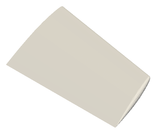
The ONERA M6 wing is a swept, semi-span wing with no twist that uses a symmetric airfoil. Widely known to aerodynamicists, the model serves as a classic reference to validate CFD methods for external flow due to its ideal combination of a simple geometry and a complex transonic flow. More information about the ONERA M6 Wing can be found at NASA’s website. The model used here has a normalized root chord of 1 m, resulting in the following geometric parameters:
Mean Aerodynamic Chord (MAC) = 0.80167 m
Semi-span = 1.47602 m
Reference area = 1.15315 m2
The mesh used for this case contains 113K nodes and 663K tetrahedrons, and the flow conditions are:
Mach Number = 0.84
Reynolds Number (based on MAC) = 11.72 Million
Alpha = 3.06°
Reference Temperature = 297.78 K
1.3.1. Upload the Mesh File#
Before uploading a mesh, install the Flow360 Python API client. Visit the API Reference section of this documentation for installation instructions. To upload a mesh and run a case, open the Python interpreter and import the Flow360 client.
python3
import flow360client
Specify no-slip boundaries - you can do this in three ways:
By directly feeding it into the
noSlipWallsargument:
noSlipWalls = [1]
By using a “*.mapbc” file:
noSlipWalls = flow360client.noSlipWallsFromMapbc('/path/to/fname.mapbc')
(Note: Make sure the boundary names in the “*.mapbc” file do NOT contain any spaces)
Or by using a
meshJsonobject:
import json
meshJson = json.load(open('/path/to/Flow360Mesh.json'))
The Flow360Mesh.json file for this tutorial has the following contents:
{
    "boundaries" :
    {
     "noSlipWalls" : [1]
    }
}
Download the mesh file from here. If using options (a) or (b), use the following command to upload the mesh:
meshId = flow360client.NewMesh(fname='/path/to/mesh.lb8.ugrid',
                               noSlipWalls=noSlipWalls,
                               meshName='my_mesh',
                               tags=[],
                               endianness='little'
                              )
If using option (c), use the following command to upload the mesh:
meshId = flow360client.NewMesh(fname='/path/to/mesh.lb8.ugrid',
                               meshJson=meshJson,
                               meshName='my_mesh',
                               tags=[],
                               endianness='little'
                              )
(Note: Arguments for meshName and tags are optional. If using a mesh filename of the format “*.lb8.ugrid” (little-endian format) or “*.b8.ugrid” (big-endian format), the endianness argument is optional. However, if you choose to use a mesh filename without “.lb8.” or “.b8.”, the endianness (‘little’ or ‘big’) must be specified appropriately in NewMesh. More information on endianness can be found here.)
Supported mesh file formats are “*.ugrid”, “*.cgns” and their “*.gz” and “*.bz2” compressions. The mesh status can be checked by using:
## to list all your mesh files
flow360client.mesh.ListMeshes()
## to view a particular mesh
flow360client.mesh.GetMeshInfo('mesh_Id')
Replace mesh_Id with your mesh’s ID.
1.3.2. Run a Case#
The Flow360.json file for this case has the following contents. A full dictionary of configuration parameters for the JSON input file can be found here.
 1{
 2    "geometry" : {
 3        "refArea" : 1.15315084119231,
 4        "momentCenter" : [0.0, 0.0, 0.0],
 5        "momentLength" : [1.47602, 0.801672958512342, 1.47602]
 6    },
 7    "volumeOutput" : {
 8        "outputFormat" : "tecplot",
 9        "animationFrequency" : -1,
10        "outputFields": ["primitiveVars", "Mach"]
11    },
12    "surfaceOutput" : {
13        "outputFormat" : "tecplot",
14        "animationFrequency" : -1,
15        "outputFields": ["primitiveVars", "Cp", "Cf"]
16    },
17    "navierStokesSolver" : {
18        "absoluteTolerance" : 1e-10,
19        "kappaMUSCL" : -1.0
20    },
21    "turbulenceModelSolver" : {
22        "modelType" : "SpalartAllmaras",
23        "absoluteTolerance" : 1e-8
24    },
25    "freestream" :
26    {
27        "Reynolds" : 14.6e6,
28        "Mach" : 0.84,
29        "Temperature" : 288.15,
30        "alphaAngle" : 3.06,
31        "betaAngle" : 0.0
32    },
33    "boundaries" : {
34        "1" : {
35		    "type" : "NoSlipWall",
36            "name" : "wing"
37		},
38		"2" : {
39			"type" : "SlipWall",
40            "name" : "symmetry"
41		},
42		"3" : {
43			"type" : "Freestream",
44            "name" : "freestream"
45		}
46    },
47    "timeStepping" : {
48        "maxPseudoSteps" : 500,
49        "CFL" : {
50            "initial" : 5,
51            "final": 200,
52            "rampSteps" : 40
53        }
54    }
55}
Use this JSON configuration file and run the case with the following command:
caseId = flow360client.NewCase(meshId='mesh_Id',
                               config='/output/path/for/Flow360.json',
                               caseName='my_case',
                               tags=[]
                              )
(Note: Arguments for caseName and tags are optional.)
The case status can be checked by using:
## to list all your cases
flow360client.case.ListCases()
## to view a particular case
flow360client.case.GetCaseInfo('case_Id')
Replace case_Id with your case’s ID.
1.3.3. Deleting a Mesh or Case#
An uploaded mesh or case can be deleted using the following commands. Caution: Cases and mesh files (including the results) cannot be recovered once deleted.
## Delete a mesh
flow360client.mesh.DeleteMesh('mesh_Id')
## Delete a case
flow360client.case.DeleteCase('case_Id')
1.3.4. Download the Results#
To download the surface data and the entire flow field, use the following command lines, respectively:
flow360client.case.DownloadSurfaceResults('case_Id', 'surfaces.tar.gz')
flow360client.case.DownloadVolumetricResults('case_Id', 'volume.tar.gz')
Once downloaded, you can postprocess these output files in either Tecplot or ParaView. You can specify the export format in the “Flow360.json” file under the volumeOutput and surfaceOutput sections.
To download the solver logs, use the following command:
flow360client.case.DownloadSolverOut('case_Id', fileName='flow360_case.user.log')
You can also download the nonlinear residuals, surface forces and total forces by using the following command line:
flow360client.case.DownloadResultsFile('case_Id', 'fileName.csv')
Replace caseId with your case’s ID and fileName with “nonlinear_residual”, “surface_forces” and “total_forces” to retrieve their respective data.
1.3.5. Visualizing the Results#
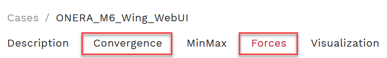
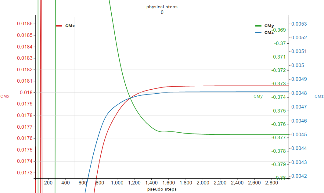
While your case is running, or after that, you can visualize the residuals and forces plots on the Web UI by clicking on your case name and viewing them under the Convergence and Forces tabs, respectively.
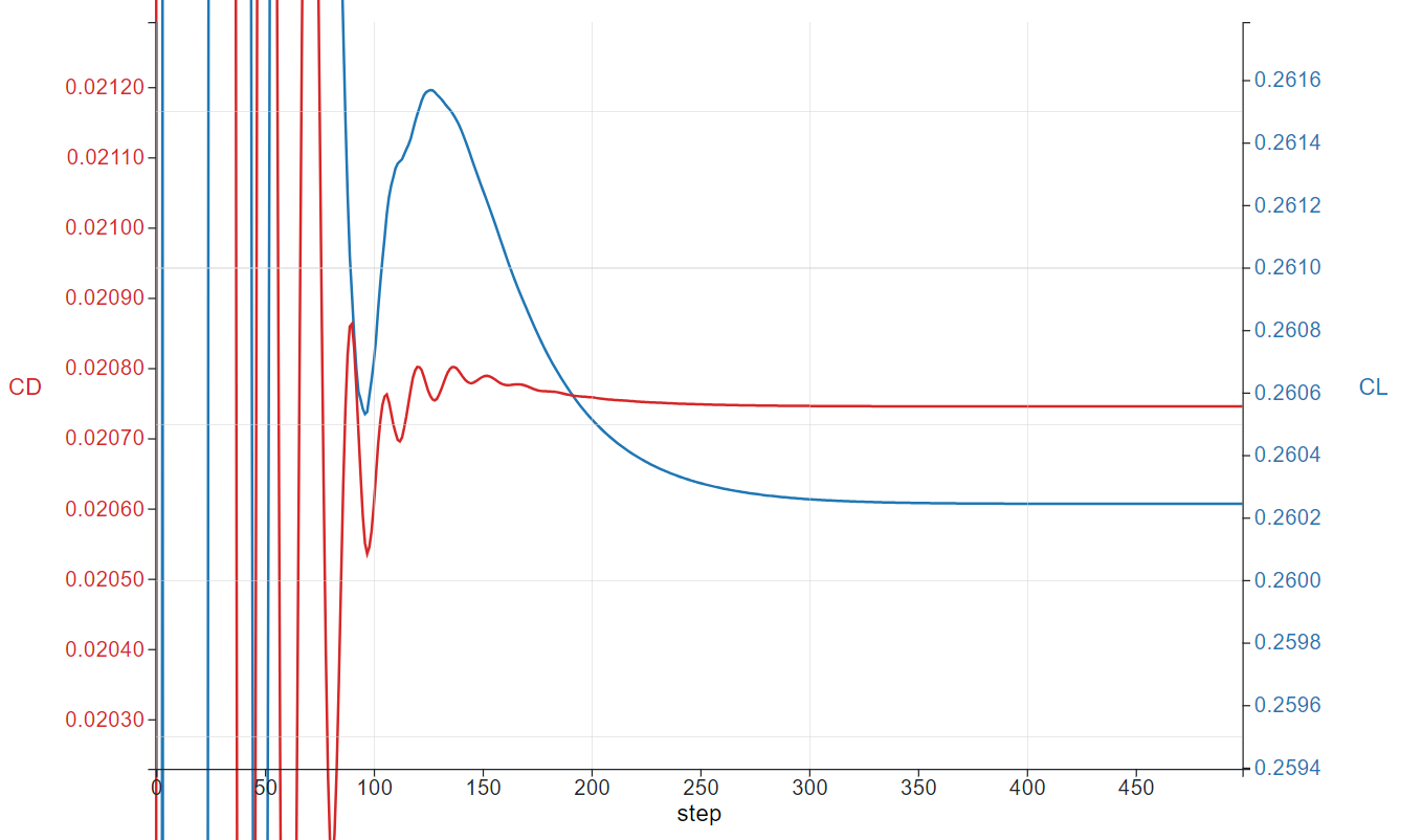
For example, the Forces plots for this case are:
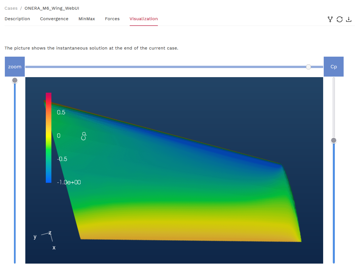
Once your case has completed running, you can also visualize the contour plots of the results under the Visualization tab. Currently, contour plots for coefficient of pressure (Cp), coefficient of skin friction (Cf), y+, and Cf with streamlines are provided.