What do I need to know about the numerical grid?#
Date |
Category |
|---|---|
2023-10-24 18:43:17 |
Grid Specification |
Tidy3D tries to provide an illusion of continuity as much as possible, but at the level of the solver, a finite numerical grid is used, which can have some implications that advanced users may want to be aware of.
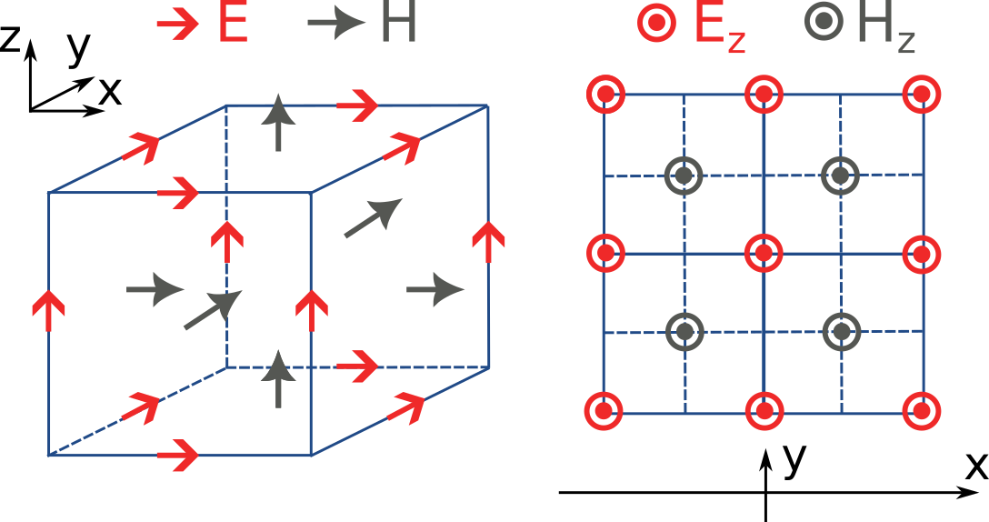
The FDTD method for electromagnetic simulations uses what is called the Yee grid, in which every field component is defined at a different spatial location, as illustrated in the figure, as well as in our FDTD video tutorial FDTD 101 videos. On the left, we show one cell of the full 3D Yee grid and where the various E and H field components live. On the right, we show a cross-section in the xy plane and the locations of the Ez and Hz field components in that plane (note that these field components are not in the same cross-section along z but rather also offset by half a cell size). This illustrates a duality between the grids on which E and H fields live, which is related to the duality between the fields themselves. There is a primal grid, shown with solid lines, and a dual grid, shown with dashed lines, with the Ez and Hz fields living at the primal/dual vertices in the xy-palne, respectively. In some literature on the FDTD method, the primal and dual grids may even be switched as the definitions are interchangeable. In Tidy3D, the primal grid is as defined by the solid lines in the Figure.
When computing results that involve multiple field components, like Poynting vector, flux, or total field intensity, it is important to use fields that are defined at the same locations for best numerical accuracy. The field components thus need to be interpolated, or colocated, to some common coordinates. All this is already done under the hood when using Tidy3D in-built methods to compute such quantities. When using field data directly, Tidy3D provides several conveniences to handle this. Firstly, field monitors have a colocate option, set to True by default, which will automatically return the field data interpolated to the primal grid vertices. The data is then ready to be used directly for computing quantities derived from any combination of the field components. The colocate option can be turned off by advanced users, in which case each field component will have different coordinates as defined by the Yee grid. In some cases, this can lead to more accurate results, as discussed, for example, in the custom source
example. In that example, when using data generated by one simulation as a source in another, it is best to use the fields as recorded on the Yee grid.
Regardless of whether the colocate option is on or off for a given monitor, the data can also be easily colocated after the solver run. In principle, if colocating to locations other than the primal grid in post-processing, it is more accurate to set colocate=False in the monitor to avoid double interpolation (first to the primal grid in the
solver, then to new locations). Regardless, the following methods work for both Yee grid data and data that has already been previously colocated:
data_at_boundaries = sim_data.at_boundaries(monitor_name)to colocate all fields of a monitor to the Yee grid cell boundaries (i.e. the primal grid vertexes).data_at_centers = sim_data.at_centers(monitor_name)to colocate all fields of a monitor to the Yee grid cell centers (i.e. the dual grid vertexes).data_at_coords = sim_data[monitor_name].colocate(x=x_points, y=y_points, z=z_points)to colocate all fields to a custom set of coordinates. Any or all ofx,y, andzcan be supplied; if some are not, the original data coordinates are kept along that dimension.