Inverse design quickstart - level 1#
This notebook will get users up and running with a very simple inverse design optimization with tidy3d. Inverse design uses the adjoint method to compute gradients of a figure of merit with respect to design parameters using only 2 simulations, no matter how many design parameters are present. This gradient is then used to do high-dimensional gradient-based optimization of the system.
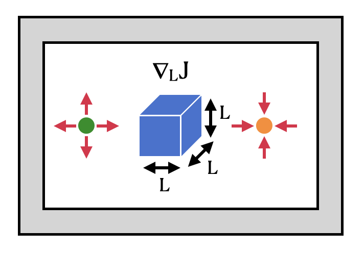
The setup we’ll demonstrate here involves a point dipole source and a point field monitor on either side of a dielectric box. We use gradient-based optimization to maximize the intensity enhancement at the measurement spot with respect to the box size in all 3 dimensions.
For more advanced inverse design examples and tutorial notebooks, check out
To see all Tidy3D examples and tutorials, as well as other learning materials, please visit our Learning Center.
[1]:
import autograd as ag
import autograd.numpy as anp
import tidy3d as td
from tidy3d.web import run
First, we define a function to create a Tidy3D Simulation given the size of the dielectric Box. We create a PointDipole source as excitation and a FieldMonitor to measure the field distribution. Later we will extract the field intensity at a point and use that as the objective function for the optimization.
[2]:
def make_sim(size_box: float) -> td.Simulation:
    """Create a tidy3d simulation given a box size."""

    # create a dipole source on the left side of the simulation
    source = td.PointDipole(
        center=(-6, 0, 0),  # position of the dipole
        source_time=td.GaussianPulse(freq0=td.C_0 / 1.55, fwidth=0.1 * td.C_0 / 1.55),
        polarization="Ez",
    )

    # create a monitor on the right side of the simulation to measure field intensity
    monitor = td.FieldMonitor(
        size=(td.inf, td.inf, 0.0),
        freqs=[td.C_0 / 1.55],
        name="field",
    )

    # create a box with the given size
    box = td.Structure(
        geometry=td.Box(center=(0, 0, 0), size=(size_box, size_box, size_box)),
        medium=td.Medium(permittivity=2),
    )

    # create the simulation
    sim = td.Simulation(
        size=(16, 16, 16),
        grid_spec=td.GridSpec.auto(min_steps_per_wvl=20),
        structures=[box],
        sources=[source],
        monitors=[monitor],
        run_time=5e-13,
    )

    return sim
Define Objective Function#
The crucial step in inverse design is to define the objective function. Now we can construct our objective function, which is simply the intensity at the measurement point \((x=6, y=0)\) as a function of the box size.
[ ]:
def objective_fn(size_box: float) -> float:
    """Calculate the intensity at the monitor position given a box size."""

    # create and run the simulation through the tidy3d web API
    sim_data = run(simulation=make_sim(size_box), task_name="adjoint_quickstart", verbose=False)

    # evaluate the intensity at the measurement position
    intensity = anp.sum(
        sim_data.get_intensity("field").sel(x=6, y=0, method="nearest").values
    )  # extract intensity at x=6 and y=0

    return intensity
Optimization Loop#
Next, we use autograd to construct a function that returns the gradient of our objective function and use this to run our gradient-based optimization in a for loop.
[4]:
# use autograd to get a function that returns the objective function and its gradient
val_and_grad_fn = ag.value_and_grad(objective_fn)

size_box = 2.5  # initial box size

# we will run the optimization for 7 iterations
for i in range(7):
    # compute gradient and current objective function value
    value, gradient = val_and_grad_fn(size_box)

    # update the parameter with the gradient and a learning rate of 2e-4
    size_box = size_box + gradient * 2e-4

    print(f"Iteration = {i + 1}\n\tsize_box = {size_box:.2f}\n\tintensity = {value:.0f}")
Iteration = 1
        size_box = 2.68
        intensity = 861
Iteration = 2
        size_box = 2.89
        intensity = 1068
Iteration = 3
        size_box = 3.07
        intensity = 1258
Iteration = 4
        size_box = 3.25
        intensity = 1402
Iteration = 5
        size_box = 3.72
        intensity = 1703
Iteration = 6
        size_box = 3.90
        intensity = 2233
Iteration = 7
        size_box = 4.08
        intensity = 2432
Analysis#
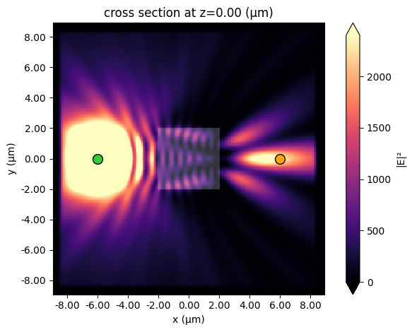
After the optimization, the final field distribution is plotted. We denote the source position with a green dot and the measurement position with an orange dot. The orange dot is near a field hotspot as a result of the optimization.
[5]:
data_final = run(simulation=make_sim(size_box), task_name="final_result", verbose=False)

# plot intensity distribution
ax = data_final.plot_field(field_monitor_name="field", field_name="E", val="abs^2", vmax=2400)

ax.plot(-6, 0, marker="o", mfc="limegreen", mec="black", ms=10)
ax.plot(6, 0, marker="o", mfc="orange", mec="black", ms=10);