Adjoint inverse design of a quantum emitter light extractor

The cost of running the entire optimization is about 8 FlexCredit (check this)

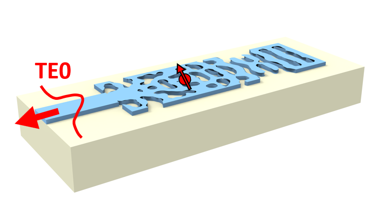
In this tutorial, we will show how to perform the adjoint-based inverse design of a quantum emitter (QE) light extraction structure. We will use a PointDipole to model the QE embedded within an integrated dielectric waveguide. Then, we will build an optimization problem to maximize the extraction efficiency of the dipole radiation into a collection waveguide. In addition, we will show how to use FieldMonitor objects in adjoint simulations to calculate the flux radiated from the dipole. You can also find helpful information in this related notebook.

If you are unfamiliar with inverse design, we recommend the inverse design lectures and this introductory tutorial.

Let’s start by importing the Python libraries used throughout this notebook.

# Standard python imports.
import pickle
from typing import List

# Import autograd for automatic differentiation.
import autograd as ag
import autograd.numpy as anp
import matplotlib.pylab as plt
import numpy as np
import optax
import scipy as sp

# Import regular tidy3d.
import tidy3d as td
import tidy3d.web as web
from tidy3d.plugins.autograd import (
    make_erosion_dilation_penalty,
    make_filter_and_project,
    rescale,
    value_and_grad,
)

Simulation Set Up

The coupling region (design region) extends a single-mode dielectric waveguide placed over a lower refractive index substrate. The QE is modeled as a PointDipole oriented in the y-direction. The QE is placed within the design region so we surround it with a constant refractive index region to protect it from etching.

# Geometric parameters.
cr_w = 1.0  # Coupling region width (um).
cr_l = 3.0  # Coupling region length (um).
wg_thick = 0.19  # Collection waveguide thickness (um).
wg_width = 0.35  # Collection waveguide width (um).
wg_length = 1.0  # Collection waveguide length (um).

# Material.
n_wg = 3.50  # Structure refractive index.
n_sub = 1.44  # Substrate refractive index.

# Fabrication constraints.
min_feature = 0.06  # Minimum feature size.
non_etch_r = 0.06  # Non-etched circular region radius (um).

# Inverse design set up parameters.
grid_size = 0.015  # Simulation grid size on design region (um).
max_iter = 100  # Maximum number of iterations.
iter_steps = 5  # Beta is increased at each iter_steps.
beta_min = 1.0  # Minimum value for the tanh projection parameter.
learning_rate = 0.02

# Simulation wavelength.
wl = 0.94  # Central simulation wavelength (um).
bw = 0.04  # Simulation bandwidth (um).
n_wl = 41  # Number of wavelength points within the bandwidth.

Let’s calculate some variables used throughout the notebook. Here, we will also define the QE position and monitor planes.

# Minimum and maximum values of the permittivity.
eps_max = n_wg**2
eps_min = 1.0

# Material definition.
mat_wg = td.Medium(permittivity=eps_max)
mat_sub = td.Medium(permittivity=n_sub**2)

# Wavelengths and frequencies.
wl_max = wl + bw / 2
wl_min = wl - bw / 2
wl_range = np.linspace(wl_min, wl_max, n_wl)
freq = td.C_0 / wl
freqs = td.C_0 / wl_range
freqw = 0.5 * (freqs[0] - freqs[-1])
run_time = 3e-12

# Computational domain size.
pml_spacing = 0.6 * wl
size_x = wg_length + cr_l + pml_spacing
size_y = cr_w + 2 * pml_spacing
size_z = wg_thick + 2 * pml_spacing
eff_inf = 10

# Source position and monitor planes.
cr_center_x = wg_length + cr_l / 2
qe_pos = td.Box(center=(cr_center_x - 0.5, 0, 0), size=(0, 0, 0))
qe_field_plan = td.Box.surfaces(center=(cr_center_x, 0, 0), size=(cr_l, cr_w, 2 * wg_thick))
wg_mode_plan = td.Box(center=(wl / 4, 0, 0), size=(0, 4 * wg_width, 5 * wg_thick))

# Number of points on design grid.
nx_grid = int(cr_l / grid_size)
ny_grid = int(cr_w / grid_size / 2)

# xy coordinates of design grid.
x_grid = np.linspace(cr_center_x - cr_l / 2, cr_center_x + cr_l / 2, nx_grid)
y_grid = np.linspace(0, cr_w / 2, ny_grid)

Optimization Set Up

We will start defining the density-based optimization functions to transform the design parameters into permittivity values. Here we include the ConicFilter, where we impose a minimum feature size fabrication constraint, and the tangent hyperbolic projection function, eliminating intermediary permittivity values as we increase the projection parameter beta. You can find more information in the Inverse design optimization of a compact grating coupler.

def pre_process(params, beta):
    filter_project = make_filter_and_project(
        radius=min_feature, dl=grid_size, beta=beta, eta=0.5, filter_type="conic"
    )
    params1 = filter_project(params, beta)
    return params1


def get_eps(params, beta: float = 1.00):
    """Returns the permittivities after filter and projection transformations"""
    params1 = pre_process(params, beta=beta)
    eps = eps_min + (eps_max - eps_min) * params1
    eps = anp.maximum(eps, eps_min)
    eps = anp.minimum(eps, eps_max)
    return eps

This function includes a circular region of constant permittivity value surrounding the QE. The objective here is to protect the QE from etching. In applications such as single photon sources, a larger unperturbed region surrounding the QE can be helpful to reduce linewidth broadening, as stated in J. Liu, K. Konthasinghe, M. Davanco, J. Lawall, V. Anant, V. Verma, R. Mirin, S. Nam, S. Woo, D. Jin, B. Ma, Z. Chen, H. Ni, Z. Niu, K. Srinivasan, "Single Self-Assembled InAs/GaAs Quantum Dots in Photonic Nanostructures: The Role of Nanofabrication," Phys. Rev. Appl. 9(6), 064019 (2018) DOI: 10.1103/PhysRevApplied.9.064019.

def include_constant_regions(eps, circ_center=[0, 0], circ_radius=1.0):
    # Build the geometric mask.
    yv, xv = anp.meshgrid(y_grid, x_grid)

    # Shouldn't this be --> |x-x0|^2 + |y-y0|^2 <= r*2
    geo_mask = (
        anp.where(
            anp.abs((xv - circ_center[0]) ** 2 + (yv - circ_center[1]) ** 2) <= (circ_radius**2),
            1,
            0,
        )
        * eps_max
    )
    eps = anp.maximum(geo_mask, eps)
    return eps

Now, we define a function to update the td.CustomMedium using the permittivity distribution. The simulation will include mirror symmetry concerning the y-direction, so only the upper half of the design region is returned by this function during the optimization process. To get the whole structure, you need to set unfold=True.

def update_design(eps, unfold=False) -> List[td.Structure]:
    # Definition of the coordinates x,y along the design region.
    coords_x = [(cr_center_x - cr_l / 2) + ix * grid_size for ix in range(nx_grid)]
    eps_val = anp.array(eps).reshape((nx_grid, ny_grid, 1))

    if not unfold:
        coords_yp = [0 + iy * grid_size for iy in range(ny_grid)]
        coords = dict(x=coords_x, y=coords_yp, z=[0])
        eps1 = td.SpatialDataArray(eps_val, coords)
        eps_medium = td.CustomMedium(permittivity=eps1)
        box = td.Box(center=(cr_center_x, cr_w / 4, 0), size=(cr_l, cr_w / 2, wg_thick))
        structure = [td.Structure(geometry=box, medium=eps_medium)]

    # VJP for one of anp.copy(), anp.concatenate(), or anp.fliplr() not defined,
    # so the optimization should only be run with `unfold=False` for now
    else:
        coords_y = [-cr_w / 2 + iy * grid_size for iy in range(2 * ny_grid)]
        coords = dict(x=coords_x, y=coords_y, z=[0])
        eps1 = td.SpatialDataArray(
            anp.concatenate((anp.fliplr(anp.copy(eps_val)), eps_val), axis=1), coords
        )
        eps_medium = td.CustomMedium(permittivity=eps1)
        box = td.Box(center=(cr_center_x, 0, 0), size=(cr_l, cr_w, wg_thick))
        structure = [td.Structure(geometry=box, medium=eps_medium)]
    return structure

In the next cell, we define the output waveguide and the substrate, as well as the simulation monitors. It is worth mentioning the inclusion of a ModeMonitor in the output waveguide and a FieldMonitor box surrounding the dipole source to calculate the total radiated power.

# Input/output waveguide.
waveguide = td.Structure(
    geometry=td.Box.from_bounds(
        rmin=(-eff_inf, -wg_width / 2, -wg_thick / 2),
        rmax=(wg_length, wg_width / 2, wg_thick / 2),
    ),
    medium=mat_wg,
)

# Substrate layer.
substrate = td.Structure(
    geometry=td.Box.from_bounds(
        rmin=(-eff_inf, -eff_inf, -eff_inf), rmax=(eff_inf, eff_inf, -wg_thick / 2)
    ),
    medium=mat_sub,
)

# Point dipole source located at the center of TiO2 thin film.
dp_source = td.PointDipole(
    center=qe_pos.center,
    source_time=td.GaussianPulse(freq0=freq, fwidth=freqw),
    polarization="Ey",
)

# Mode monitor to compute the FOM.
mode_spec = td.ModeSpec(num_modes=1, target_neff=n_wg)
mode_monitor_fom = td.ModeMonitor(
    center=wg_mode_plan.center,
    size=wg_mode_plan.size,
    freqs=[freq],
    mode_spec=mode_spec,
    name="mode_monitor_fom",
)

# Field monitor to compute the FOM.
field_monitor_fom = []
for i, plane in enumerate(qe_field_plan):
    field_monitor_fom.append(
        td.FieldMonitor(
            center=plane.center,
            size=plane.size,
            freqs=[freq],
            name=f"field_monitor_fom_{i}",
        )
    )

# Mode monitor to compute spectral response.
mode_spec = td.ModeSpec(num_modes=1, target_neff=n_wg)
mode_monitor = td.ModeMonitor(
    center=wg_mode_plan.center,
    size=wg_mode_plan.size,
    freqs=freqs,
    mode_spec=mode_spec,
    name="mode_monitor",
)

# Field monitor to compute spectral response.
field_monitor = []
for i, plane in enumerate(qe_field_plan):
    field_monitor.append(
        td.FieldMonitor(
            center=plane.center, size=plane.size, freqs=freqs, name=f"field_monitor_{i}"
        )
    )

# Field monitor to visualize the fields.
field_monitor_xy = td.FieldMonitor(
    center=(size_x / 2, 0, 0),
    size=(size_x, size_y, 0),
    freqs=freqs,
    name="field_xy",
)

Lastly, we have a function that receives the design parameters from the optimization algorithm and then gathers the simulation objects altogether to create a td.Simulation.

def make_adjoint_sim(param, beta: float = 1.00, unfold=False):
    eps = get_eps(param, beta)
    eps = include_constant_regions(
        eps, circ_center=[qe_pos.center[0], qe_pos.center[1]], circ_radius=non_etch_r
    )
    structure = update_design(eps, unfold=unfold)

    # Creates a uniform mesh for the design region.
    adjoint_dr_mesh = td.MeshOverrideStructure(
        geometry=td.Box(center=(cr_center_x, 0, 0), size=(cr_w, cr_l, wg_thick)),
        dl=[grid_size, grid_size, grid_size],
        enforce=True,
    )

    grid_spec = td.GridSpec.auto(
        wavelength=wl_max,
        min_steps_per_wvl=15,
        override_structures=[adjoint_dr_mesh],
    )

    return td.Simulation(
        size=[size_x, size_y, size_z],
        center=[size_x / 2, 0, 0],
        grid_spec=grid_spec,
        symmetry=(0, -1, 0),
        structures=[substrate, waveguide] + structure,
        sources=[dp_source],
        monitors=[field_monitor_xy, mode_monitor_fom] + field_monitor_fom,
        run_time=run_time,
        subpixel=True,
    )

Initial Light Extractor Structure

Let’s create a uniform initial permittivity distribution and verify if all the simulation objects are in the correct places.

init_par = np.ones((nx_grid, ny_grid)) * 0.5
init_design = make_adjoint_sim(init_par, beta=beta_min, unfold=True)

fig, (ax1, ax2) = plt.subplots(1, 2, tight_layout=True, figsize=(12, 4))
init_design.plot_eps(z=0, ax=ax1, monitor_alpha=0.0)
init_design.plot_eps(y=0, ax=ax2)
plt.show()

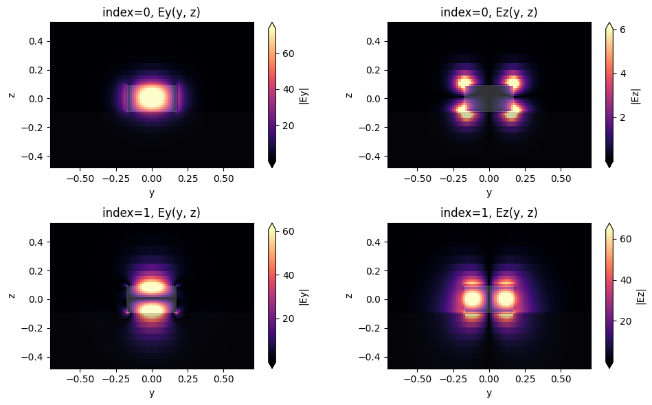
We will also look at the collection waveguide mode to ensure we have considered the correct one in the ModeMonitor setup. We use the ModeSolver plugin to calculate the first two waveguide modes, as below.

from tidy3d.plugins.mode import ModeSolver
from tidy3d.plugins.mode.web import run as run_mode_solver

sim_init = init_design.updated_copy(monitors=[field_monitor_xy, mode_monitor] + field_monitor)

mode_solver = ModeSolver(
    simulation=sim_init,
    plane=wg_mode_plan,
    mode_spec=td.ModeSpec(num_modes=2),
    freqs=[freq],
)
modes = run_mode_solver(mode_solver, reduce_simulation=True)

16:10:23 CEST Mode solver created with
              task_id='fdve-65e65354-aedf-458c-a514-a7eccc5e4b24',
              solver_id='mo-581ee868-4940-489c-bab0-2c43f11c8df2'.

16:10:26 CEST Mode solver status: queued

16:10:28 CEST Mode solver status: running

16:10:32 CEST Mode solver status: success

After inspecting the mode field distribution, we can confirm that the fundamental waveguide mode is mainly oriented in the y-direction, thus matching the dipole orientation.

fig, axs = plt.subplots(2, 2, figsize=(10, 6), tight_layout=True)
for mode_ind in range(2):
    for field_ind, field_name in enumerate(("Ey", "Ez")):
        ax = axs[mode_ind, field_ind]
        mode_solver.plot_field(field_name, "abs", mode_index=mode_ind, f=freq, ax=ax)
        ax.set_title(f"index={mode_ind}, {field_name}(y, z)")

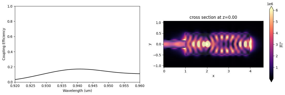
Then, we will calculate the initial coupling efficiency to see how this random structure performs.

sim_data = web.run(sim_init, task_name="initial QE light extractor (Autograd)")

16:10:35 CEST Created task 'initial QE light extractor (Autograd)' with task_id
              'fdve-4ca772ae-badc-4827-8da8-4b32cf325ab4' and task_type 'FDTD'.

              View task using web UI at
              'https://tidy3d.simulation.cloud/workbench?taskId=fdve-4ca772ae-ba
              dc-4827-8da8-4b32cf325ab4'.

              Task folder: 'default'.

16:10:37 CEST Maximum FlexCredit cost: 0.060. Minimum cost depends on task
              execution details. Use 'web.real_cost(task_id)' to get the billed
              FlexCredit cost after a simulation run.

16:10:38 CEST status = success

16:10:43 CEST loading simulation from simulation_data.hdf5

The modal coupling efficiency is normalized by the dipole power. That is necessary because the dipole power will likely change significantly when the optimization algorithm modifies the design region.

mode_amps = sim_data["mode_monitor"].amps.sel(direction="-", mode_index=0)
mode_power = np.abs(mode_amps) ** 2
dip_power = np.zeros(n_wl)
for i in range(len(field_monitor)):
    field_mon = sim_data[f"field_monitor_{i}"]
    dip_power += np.abs(field_mon.flux)

coup_eff = mode_power / dip_power

f, (ax1, ax2) = plt.subplots(1, 2, figsize=(12, 4), tight_layout=True)
ax1.plot(wl_range, coup_eff, "-k")
ax1.set_xlabel("Wavelength (um)")
ax1.set_ylabel("Coupling Efficiency")
ax1.set_ylim(0, 1)
ax1.set_xlim(wl - bw / 2, wl + bw / 2)
sim_data.plot_field("field_xy", "E", "abs^2", z=0, ax=ax2, f=freq)
plt.show()

Optimization

The objective function defined next is the device figure-of-merit (FOM) minus a fabrication penalty.

# Figure of Merit (FOM) calculation.
def fom(sim_data: td.SimulationData) -> float:
    """Return the coupling efficiency."""
    # best to use autograd-wrapped numpy functions for differentiation
    mode_amps = sim_data["mode_monitor_fom"].amps.sel(direction="-", f=freq, mode_index=0).data
    mode_power = anp.sum(anp.abs(mode_amps) ** 2)

    # unlike Jax version, should avoid in-place operators (e.g, `+=`), use numpy when possible
    field_mon_list = [sim_data[f"field_monitor_fom_{i}"] for i in range(0, 6)]
    dip_power = anp.sum([anp.abs(mon.flux.data) for mon in field_mon_list])

    return mode_power, dip_power


def penalty(params, beta) -> float:
    """Penalize changes in structure after erosion and dilation to enforce larger feature sizes."""
    params_processed = pre_process(params, beta=beta)
    erode_dilate_penalty = make_erosion_dilation_penalty(radius=min_feature, dl=grid_size)
    ed_penalty = erode_dilate_penalty(params_processed)
    return ed_penalty


# Objective function to be passed to the optimization algorithm.
def obj(param, beta: float = 1.0, step_num: int = None, verbose: bool = False) -> float:
    sim = make_adjoint_sim(param, beta, unfold=False)  # non-differentiable if `unfold=True`
    task_name = "inv_des"
    if step_num:
        task_name += f"_step_{step_num}"
    sim_data = web.run(sim, task_name=task_name, verbose=verbose)
    mode_power, dip_power = fom(sim_data)
    fom_val = mode_power / dip_power
    penalty_weight = 0.1
    penalty_val = penalty(param, beta)
    J = fom_val - penalty_weight * penalty_val
    return J, [sim_data, mode_power, dip_power, penalty_val]


# Function to calculate the objective function value and its gradient with respect to the design parameters.
# Use tidy3d's wrapped ag.value_and_grad() for it's auxiliary data functionality
obj_grad = value_and_grad(obj, has_aux=True)

In the following cell, we define some functions to save the optimization progress and load a previous optimization from the file.

# where to store history
history_fname = "misc/qe_light_coupler_autograd.pkl"


def save_history(history_dict: dict) -> None:
    """Convenience function to save the history to file."""
    with open(history_fname, "wb") as file:
        pickle.dump(history_dict, file)


def load_history() -> dict:
    """Convenience method to load the history from file."""
    with open(history_fname, "rb") as file:
        history_dict = pickle.load(file)
    return history_dict

Then, we will start a new optimization or load the parameters of a previous one.

# initialize adam optimizer with starting parameters
optimizer = optax.adam(learning_rate=learning_rate)

try:
    history_dict = load_history()
    opt_state = history_dict["opt_states"][-1]
    params = history_dict["params"][-1]
    opt_state = optimizer.init(params)
    num_iters_completed = len(history_dict["params"])
    print("Loaded optimization checkpoint from file.")
    print(f"Found {num_iters_completed} iterations previously completed out of {max_iter} total.")
    if num_iters_completed < max_iter:
        print("Will resume optimization.")
    else:
        print("Optimization completed, will return results.")

except FileNotFoundError:
    params = anp.array(init_par)
    opt_state = optimizer.init(params)
    history_dict = dict(
        values=[],
        coupl_eff=[],
        penalty=[],
        params=[],
        gradients=[],
        opt_states=[opt_state],
        data=[],
        beta=[],
    )

WARNING:2025-07-26 16:10:43,499:jax._src.xla_bridge:967: An NVIDIA GPU may be present on this machine, but a CUDA-enabled jaxlib is not installed. Falling back to cpu.

In the optimization loop, we will gradually increase the projection parameter beta to eliminate intermediary permittivity values. At each iteration, we record the design parameters and the optimization history to restore them as needed.

iter_done = len(history_dict["values"])
if iter_done < max_iter:
    # small # of iters for quick testing
    for i in range(iter_done, max_iter):
        print(f"Iteration = ({i + 1} / {max_iter})")
        plt.subplots(1, 1, figsize=(3, 2))
        plt.imshow(np.flipud(1 - params.T), cmap="gray", vmin=0, vmax=1)
        plt.axis("off")
        plt.show()

        # Compute gradient and current objective function value.
        beta_i = i // iter_steps + beta_min
        (value, gradient), data = obj_grad(params, beta=beta_i, step_num=(i + 1))
        sim_data_i, mode_power_i, dip_power_i, penalty_val_i = [data[0]] + [
            dat._value for dat in data[1:]
        ]
        # Outputs.
        print(f"\tbeta = {beta_i}")
        print(f"\tJ = {value:.4e}")
        print(f"\tgrad_norm = {np.linalg.norm(gradient):.4e}")
        print(f"\tpenalty = {penalty_val_i:.3f}")
        print(f"\tmode power = {mode_power_i:.3f}")
        print(f"\tdip power = {dip_power_i:.3f}")
        print(f"\tcoupling efficiency = {mode_power_i / dip_power_i:.3f}")

        # Compute and apply updates to the optimizer based on gradient (-1 sign to maximize obj_fn).
        updates, opt_state = optimizer.update(-gradient, opt_state, params)
        params = optax.apply_updates(params, updates)

        # Cap parameters between 0 and 1.
        params = anp.minimum(params, 1.0)
        params = anp.maximum(params, 0.0)

        # Save history.
        history_dict["values"].append(value)
        history_dict["coupl_eff"].append(mode_power_i / dip_power_i)
        history_dict["penalty"].append(penalty_val_i)
        history_dict["params"].append(params)
        history_dict["beta"].append(beta_i)
        history_dict["gradients"].append(gradient)
        history_dict["opt_states"].append(opt_state)
        # history_dict["data"].append(sim_data_i)  # Uncomment to store data, can create large files.
        save_history(history_dict)

Iteration = (1 / 100)

        beta = 1.0
        J = 7.1432e-02
        grad_norm = 6.8739e-02
        penalty = 1.000
        mode power = 473.968
        dip power = 2764.752
        coupling efficiency = 0.171
Iteration = (2 / 100)

        beta = 1.0
        J = 2.2832e-01
        grad_norm = 7.1512e-02
        penalty = 1.000
        mode power = 1002.394
        dip power = 3053.089
        coupling efficiency = 0.328
Iteration = (3 / 100)

        beta = 1.0
        J = 3.7482e-01
        grad_norm = 6.4898e-02
        penalty = 1.000
        mode power = 1478.833
        dip power = 3114.501
        coupling efficiency = 0.475
Iteration = (4 / 100)

        beta = 1.0
        J = 4.9571e-01
        grad_norm = 5.6425e-02
        penalty = 1.000
        mode power = 1935.575
        dip power = 3249.175
        coupling efficiency = 0.596
Iteration = (5 / 100)

        beta = 1.0
        J = 5.8980e-01
        grad_norm = 4.6824e-02
        penalty = 1.000
        mode power = 2418.556
        dip power = 3506.185
        coupling efficiency = 0.690
Iteration = (6 / 100)

        beta = 2.0
        J = 6.9596e-01
        grad_norm = 5.4160e-02
        penalty = 1.000
        mode power = 3059.636
        dip power = 3843.981
        coupling efficiency = 0.796
Iteration = (7 / 100)

        beta = 2.0
        J = 7.4070e-01
        grad_norm = 3.8978e-02
        penalty = 1.000
        mode power = 3716.945
        dip power = 4421.261
        coupling efficiency = 0.841
Iteration = (8 / 100)

        beta = 2.0
        J = 7.7138e-01
        grad_norm = 3.0304e-02
        penalty = 1.000
        mode power = 4429.873
        dip power = 5083.755
        coupling efficiency = 0.871
Iteration = (9 / 100)

        beta = 2.0
        J = 7.9249e-01
        grad_norm = 2.9056e-02
        penalty = 1.000
        mode power = 5169.262
        dip power = 5791.995
        coupling efficiency = 0.892
Iteration = (10 / 100)

        beta = 2.0
        J = 8.0856e-01
        grad_norm = 2.8136e-02
        penalty = 1.000
        mode power = 6042.956
        dip power = 6651.128
        coupling efficiency = 0.909
Iteration = (11 / 100)

        beta = 3.0
        J = 7.9742e-01
        grad_norm = 9.7527e-02
        penalty = 1.000
        mode power = 7003.191
        dip power = 7803.999
        coupling efficiency = 0.897
Iteration = (12 / 100)

        beta = 3.0
        J = 8.3259e-01
        grad_norm = 3.7221e-02
        penalty = 0.999
        mode power = 8407.922
        dip power = 9016.226
        coupling efficiency = 0.933
Iteration = (13 / 100)

        beta = 3.0
        J = 8.2696e-01
        grad_norm = 6.7464e-02
        penalty = 0.999
        mode power = 8736.356
        dip power = 9425.743
        coupling efficiency = 0.927
Iteration = (14 / 100)

        beta = 3.0
        J = 8.1778e-01
        grad_norm = 1.0335e-01
        penalty = 0.999
        mode power = 8016.955
        dip power = 8736.591
        coupling efficiency = 0.918
Iteration = (15 / 100)

        beta = 3.0
        J = 8.3701e-01
        grad_norm = 7.7907e-02
        penalty = 0.998
        mode power = 7685.024
        dip power = 8203.539
        coupling efficiency = 0.937
Iteration = (16 / 100)

        beta = 4.0
        J = 8.1204e-01
        grad_norm = 1.5668e-01
        penalty = 0.983
        mode power = 5820.384
        dip power = 6393.784
        coupling efficiency = 0.910
Iteration = (17 / 100)

        beta = 4.0
        J = 8.4011e-01
        grad_norm = 1.0337e-01
        penalty = 0.977
        mode power = 7501.458
        dip power = 7998.690
        coupling efficiency = 0.938
Iteration = (18 / 100)

        beta = 4.0
        J = 8.6124e-01
        grad_norm = 2.8364e-02
        penalty = 0.971
        mode power = 10468.018
        dip power = 10923.463
        coupling efficiency = 0.958
Iteration = (19 / 100)

        beta = 4.0
        J = 8.5361e-01
        grad_norm = 7.5763e-02
        penalty = 0.963
        mode power = 13775.781
        dip power = 14501.615
        coupling efficiency = 0.950
Iteration = (20 / 100)

        beta = 4.0
        J = 8.5295e-01
        grad_norm = 8.1482e-02
        penalty = 0.956
        mode power = 16346.014
        dip power = 17233.051
        coupling efficiency = 0.949
Iteration = (21 / 100)

        beta = 5.0
        J = 8.7218e-01
        grad_norm = 5.7052e-02
        penalty = 0.875
        mode power = 17111.887
        dip power = 17829.989
        coupling efficiency = 0.960
Iteration = (22 / 100)

        beta = 5.0
        J = 8.8005e-01
        grad_norm = 5.3833e-02
        penalty = 0.865
        mode power = 17308.501
        dip power = 17908.051
        coupling efficiency = 0.967
Iteration = (23 / 100)

        beta = 5.0
        J = 8.8289e-01
        grad_norm = 3.2505e-02
        penalty = 0.854
        mode power = 15082.259
        dip power = 15576.252
        coupling efficiency = 0.968
Iteration = (24 / 100)

        beta = 5.0
        J = 8.8113e-01
        grad_norm = 4.4331e-02
        penalty = 0.843
        mode power = 12419.322
        dip power = 12863.968
        coupling efficiency = 0.965
Iteration = (25 / 100)

        beta = 5.0
        J = 8.7947e-01
        grad_norm = 6.3651e-02
        penalty = 0.832
        mode power = 12087.040
        dip power = 12555.809
        coupling efficiency = 0.963
Iteration = (26 / 100)

        beta = 6.0
        J = 8.8584e-01
        grad_norm = 7.8859e-02
        penalty = 0.732
        mode power = 10924.212
        dip power = 11390.265
        coupling efficiency = 0.959
Iteration = (27 / 100)

        beta = 6.0
        J = 8.9808e-01
        grad_norm = 3.3468e-02
        penalty = 0.722
        mode power = 17336.079
        dip power = 17867.154
        coupling efficiency = 0.970
Iteration = (28 / 100)

        beta = 6.0
        J = 9.0230e-01
        grad_norm = 7.8044e-02
        penalty = 0.712
        mode power = 25590.844
        dip power = 26288.327
        coupling efficiency = 0.973
Iteration = (29 / 100)

        beta = 6.0
        J = 8.9802e-01
        grad_norm = 9.3922e-02
        penalty = 0.702
        mode power = 26559.148
        dip power = 27429.898
        coupling efficiency = 0.968
Iteration = (30 / 100)

        beta = 6.0
        J = 8.9534e-01
        grad_norm = 7.9459e-02
        penalty = 0.694
        mode power = 21200.802
        dip power = 21975.043
        coupling efficiency = 0.965
Iteration = (31 / 100)

        beta = 7.0
        J = 8.9894e-01
        grad_norm = 1.4495e-01
        penalty = 0.610
        mode power = 11024.127
        dip power = 11483.994
        coupling efficiency = 0.960
Iteration = (32 / 100)

        beta = 7.0
        J = 9.0821e-01
        grad_norm = 7.0287e-02
        penalty = 0.604
        mode power = 15566.298
        dip power = 16071.417
        coupling efficiency = 0.969
Iteration = (33 / 100)

        beta = 7.0
        J = 9.0284e-01
        grad_norm = 1.1942e-01
        penalty = 0.597
        mode power = 24449.286
        dip power = 25399.992
        coupling efficiency = 0.963
Iteration = (34 / 100)

        beta = 7.0
        J = 9.0576e-01
        grad_norm = 1.2081e-01
        penalty = 0.591
        mode power = 25232.320
        dip power = 26150.739
        coupling efficiency = 0.965
Iteration = (35 / 100)

        beta = 7.0
        J = 9.1589e-01
        grad_norm = 4.2125e-02
        penalty = 0.585
        mode power = 18147.493
        dip power = 18623.626
        coupling efficiency = 0.974
Iteration = (36 / 100)

        beta = 8.0
        J = 9.1102e-01
        grad_norm = 1.3288e-01
        penalty = 0.522
        mode power = 8422.290
        dip power = 8743.769
        coupling efficiency = 0.963
Iteration = (37 / 100)

        beta = 8.0
        J = 9.1466e-01
        grad_norm = 1.2887e-01
        penalty = 0.518
        mode power = 11193.142
        dip power = 11582.000
        coupling efficiency = 0.966
Iteration = (38 / 100)

        beta = 8.0
        J = 9.2233e-01
        grad_norm = 4.5024e-02
        penalty = 0.514
        mode power = 22909.328
        dip power = 23528.628
        coupling efficiency = 0.974
Iteration = (39 / 100)

        beta = 8.0
        J = 9.1957e-01
        grad_norm = 1.8263e-01
        penalty = 0.510
        mode power = 33641.288
        dip power = 34663.037
        coupling efficiency = 0.971
Iteration = (40 / 100)

        beta = 8.0
        J = 9.2188e-01
        grad_norm = 9.1393e-02
        penalty = 0.505
        mode power = 29094.673
        dip power = 29920.135
        coupling efficiency = 0.972
Iteration = (41 / 100)

        beta = 9.0
        J = 9.1973e-01
        grad_norm = 1.7000e-01
        penalty = 0.458
        mode power = 10998.133
        dip power = 11390.796
        coupling efficiency = 0.966
Iteration = (42 / 100)

        beta = 9.0
        J = 9.2859e-01
        grad_norm = 9.8428e-02
        penalty = 0.454
        mode power = 11288.366
        dip power = 11589.890
        coupling efficiency = 0.974
Iteration = (43 / 100)

        beta = 9.0
        J = 9.2298e-01
        grad_norm = 1.3906e-01
        penalty = 0.450
        mode power = 16924.833
        dip power = 17484.737
        coupling efficiency = 0.968
Iteration = (44 / 100)

        beta = 9.0
        J = 9.2668e-01
        grad_norm = 1.0958e-01
        penalty = 0.446
        mode power = 28103.075
        dip power = 28934.711
        coupling efficiency = 0.971
Iteration = (45 / 100)

        beta = 9.0
        J = 9.2947e-01
        grad_norm = 1.2422e-01
        penalty = 0.441
        mode power = 35342.692
        dip power = 36301.386
        coupling efficiency = 0.974
Iteration = (46 / 100)

        beta = 10.0
        J = 9.1725e-01
        grad_norm = 2.0425e-01
        penalty = 0.402
        mode power = 22519.909
        dip power = 23521.792
        coupling efficiency = 0.957
Iteration = (47 / 100)

        beta = 10.0
        J = 9.3295e-01
        grad_norm = 8.7255e-02
        penalty = 0.397
        mode power = 27879.178
        dip power = 28662.293
        coupling efficiency = 0.973
Iteration = (48 / 100)

        beta = 10.0
        J = 9.2987e-01
        grad_norm = 1.6063e-01
        penalty = 0.393
        mode power = 36241.082
        dip power = 37392.982
        coupling efficiency = 0.969
Iteration = (49 / 100)

        beta = 10.0
        J = 9.3010e-01
        grad_norm = 1.5227e-01
        penalty = 0.388
        mode power = 34755.844
        dip power = 35869.977
        coupling efficiency = 0.969
Iteration = (50 / 100)

        beta = 10.0
        J = 9.3480e-01
        grad_norm = 8.6082e-02
        penalty = 0.383
        mode power = 24952.972
        dip power = 25642.153
        coupling efficiency = 0.973
Iteration = (51 / 100)

        beta = 11.0
        J = 9.2062e-01
        grad_norm = 2.6132e-01
        penalty = 0.353
        mode power = 14742.606
        dip power = 15421.940
        coupling efficiency = 0.956
Iteration = (52 / 100)

        beta = 11.0
        J = 9.3850e-01
        grad_norm = 6.0557e-02
        penalty = 0.351
        mode power = 30944.033
        dip power = 31783.785
        coupling efficiency = 0.974
Iteration = (53 / 100)

        beta = 11.0
        J = 9.2657e-01
        grad_norm = 4.5544e-01
        penalty = 0.349
        mode power = 62661.433
        dip power = 65175.091
        coupling efficiency = 0.961
Iteration = (54 / 100)

        beta = 11.0
        J = 9.3726e-01
        grad_norm = 1.3739e-01
        penalty = 0.344
        mode power = 26083.433
        dip power = 26843.055
        coupling efficiency = 0.972
Iteration = (55 / 100)

        beta = 11.0
        J = 9.3110e-01
        grad_norm = 2.7552e-01
        penalty = 0.340
        mode power = 14073.962
        dip power = 14582.365
        coupling efficiency = 0.965
Iteration = (56 / 100)

        beta = 12.0
        J = 9.3442e-01
        grad_norm = 2.0789e-01
        penalty = 0.318
        mode power = 10793.581
        dip power = 11171.070
        coupling efficiency = 0.966
Iteration = (57 / 100)

        beta = 12.0
        J = 9.3674e-01
        grad_norm = 2.0010e-01
        penalty = 0.316
        mode power = 24160.809
        dip power = 24951.189
        coupling efficiency = 0.968
Iteration = (58 / 100)

        beta = 12.0
        J = 9.3609e-01
        grad_norm = 4.0679e-01
        penalty = 0.314
        mode power = 70509.692
        dip power = 72879.455
        coupling efficiency = 0.967
Iteration = (59 / 100)

        beta = 12.0
        J = 9.3791e-01
        grad_norm = 2.0113e-01
        penalty = 0.311
        mode power = 41804.340
        dip power = 43143.020
        coupling efficiency = 0.969
Iteration = (60 / 100)

        beta = 12.0
        J = 9.4025e-01
        grad_norm = 2.5264e-01
        penalty = 0.307
        mode power = 25748.521
        dip power = 26517.867
        coupling efficiency = 0.971
Iteration = (61 / 100)

        beta = 13.0
        J = 9.4298e-01
        grad_norm = 1.9770e-01
        penalty = 0.289
        mode power = 18771.299
        dip power = 19314.514
        coupling efficiency = 0.972
Iteration = (62 / 100)

        beta = 13.0
        J = 9.3831e-01
        grad_norm = 2.4655e-01
        penalty = 0.286
        mode power = 36051.354
        dip power = 37283.141
        coupling efficiency = 0.967
Iteration = (63 / 100)

        beta = 13.0
        J = 9.4770e-01
        grad_norm = 3.0916e-01
        penalty = 0.284
        mode power = 73330.091
        dip power = 75124.741
        coupling efficiency = 0.976
Iteration = (64 / 100)

        beta = 13.0
        J = 9.4116e-01
        grad_norm = 2.3562e-01
        penalty = 0.281
        mode power = 48064.009
        dip power = 49586.843
        coupling efficiency = 0.969
Iteration = (65 / 100)

        beta = 13.0
        J = 9.4345e-01
        grad_norm = 2.5314e-01
        penalty = 0.279
        mode power = 34732.187
        dip power = 35758.010
        coupling efficiency = 0.971
Iteration = (66 / 100)

        beta = 14.0
        J = 9.5072e-01
        grad_norm = 1.4767e-01
        penalty = 0.264
        mode power = 28125.287
        dip power = 28783.696
        coupling efficiency = 0.977
Iteration = (67 / 100)

        beta = 14.0
        J = 9.4194e-01
        grad_norm = 2.4715e-01
        penalty = 0.262
        mode power = 46559.660
        dip power = 48091.621
        coupling efficiency = 0.968
Iteration = (68 / 100)

        beta = 14.0
        J = 9.4917e-01
        grad_norm = 2.2277e-01
        penalty = 0.260
        mode power = 72396.961
        dip power = 74239.709
        coupling efficiency = 0.975
Iteration = (69 / 100)

        beta = 14.0
        J = 9.4340e-01
        grad_norm = 2.4728e-01
        penalty = 0.258
        mode power = 50687.983
        dip power = 52298.049
        coupling efficiency = 0.969
Iteration = (70 / 100)

        beta = 14.0
        J = 9.4637e-01
        grad_norm = 2.1213e-01
        penalty = 0.256
        mode power = 46727.818
        dip power = 48073.883
        coupling efficiency = 0.972
Iteration = (71 / 100)

        beta = 15.0
        J = 9.4793e-01
        grad_norm = 2.0206e-01
        penalty = 0.245
        mode power = 43807.749
        dip power = 45051.273
        coupling efficiency = 0.972
Iteration = (72 / 100)

        beta = 15.0
        J = 9.4802e-01
        grad_norm = 2.3269e-01
        penalty = 0.243
        mode power = 65613.204
        dip power = 67481.891
        coupling efficiency = 0.972
Iteration = (73 / 100)

        beta = 15.0
        J = 9.4520e-01
        grad_norm = 2.0955e-01
        penalty = 0.241
        mode power = 58289.876
        dip power = 60136.353
        coupling efficiency = 0.969
Iteration = (74 / 100)

        beta = 15.0
        J = 9.4843e-01
        grad_norm = 1.9381e-01
        penalty = 0.239
        mode power = 59574.966
        dip power = 61270.094
        coupling efficiency = 0.972
Iteration = (75 / 100)

        beta = 15.0
        J = 9.4856e-01
        grad_norm = 1.8808e-01
        penalty = 0.237
        mode power = 71769.585
        dip power = 73817.117
        coupling efficiency = 0.972
Iteration = (76 / 100)

        beta = 16.0
        J = 9.4920e-01
        grad_norm = 2.2412e-01
        penalty = 0.227
        mode power = 34792.815
        dip power = 35798.471
        coupling efficiency = 0.972
Iteration = (77 / 100)

        beta = 16.0
        J = 9.5233e-01
        grad_norm = 1.1844e-01
        penalty = 0.225
        mode power = 49022.100
        dip power = 50286.898
        coupling efficiency = 0.975
Iteration = (78 / 100)

        beta = 16.0
        J = 9.4676e-01
        grad_norm = 4.5962e-01
        penalty = 0.223
        mode power = 112223.050
        dip power = 115803.635
        coupling efficiency = 0.969
Iteration = (79 / 100)

        beta = 16.0
        J = 9.5146e-01
        grad_norm = 2.6840e-01
        penalty = 0.222
        mode power = 24794.677
        dip power = 25465.193
        coupling efficiency = 0.974
Iteration = (80 / 100)

        beta = 16.0
        J = 9.4763e-01
        grad_norm = 2.8706e-01
        penalty = 0.221
        mode power = 20580.707
        dip power = 21223.601
        coupling efficiency = 0.970
Iteration = (81 / 100)

        beta = 17.0
        J = 9.4846e-01
        grad_norm = 2.7118e-01
        penalty = 0.213
        mode power = 26519.913
        dip power = 27347.167
        coupling efficiency = 0.970
Iteration = (82 / 100)

        beta = 17.0
        J = 9.4705e-01
        grad_norm = 2.4277e-01
        penalty = 0.211
        mode power = 83580.160
        dip power = 86326.033
        coupling efficiency = 0.968
Iteration = (83 / 100)

        beta = 17.0
        J = 9.4165e-01
        grad_norm = 4.2922e-01
        penalty = 0.210
        mode power = 107209.997
        dip power = 111366.379
        coupling efficiency = 0.963
Iteration = (84 / 100)

        beta = 17.0
        J = 9.5012e-01
        grad_norm = 2.7870e-01
        penalty = 0.210
        mode power = 26200.887
        dip power = 26981.020
        coupling efficiency = 0.971
Iteration = (85 / 100)

        beta = 17.0
        J = 9.4240e-01
        grad_norm = 3.2850e-01
        penalty = 0.209
        mode power = 22240.250
        dip power = 23088.709
        coupling efficiency = 0.963
Iteration = (86 / 100)

        beta = 18.0
        J = 9.4756e-01
        grad_norm = 2.9047e-01
        penalty = 0.202
        mode power = 21835.585
        dip power = 22562.989
        coupling efficiency = 0.968
Iteration = (87 / 100)

        beta = 18.0
        J = 9.4655e-01
        grad_norm = 2.8581e-01
        penalty = 0.201
        mode power = 44635.553
        dip power = 46177.909
        coupling efficiency = 0.967
Iteration = (88 / 100)

        beta = 18.0
        J = 9.4568e-01
        grad_norm = 1.4660e+00
        penalty = 0.198
        mode power = 191151.713
        dip power = 197978.584
        coupling efficiency = 0.966
Iteration = (89 / 100)

        beta = 18.0
        J = 9.0565e-01
        grad_norm = 7.1548e-01
        penalty = 0.200
        mode power = 7787.385
        dip power = 8413.092
        coupling efficiency = 0.926
Iteration = (90 / 100)

        beta = 18.0
        J = 9.1608e-01
        grad_norm = 5.4755e-01
        penalty = 0.200
        mode power = 3829.103
        dip power = 4090.553
        coupling efficiency = 0.936
Iteration = (91 / 100)

        beta = 19.0
        J = 9.1000e-01
        grad_norm = 4.0796e-01
        penalty = 0.196
        mode power = 3154.019
        dip power = 3393.009
        coupling efficiency = 0.930
Iteration = (92 / 100)

        beta = 19.0
        J = 8.9532e-01
        grad_norm = 4.8212e-01
        penalty = 0.196
        mode power = 3168.027
        dip power = 3462.783
        coupling efficiency = 0.915
Iteration = (93 / 100)

        beta = 19.0
        J = 9.1045e-01
        grad_norm = 3.6817e-01
        penalty = 0.196
        mode power = 3353.528
        dip power = 3605.939
        coupling efficiency = 0.930
Iteration = (94 / 100)

        beta = 19.0
        J = 9.3083e-01
        grad_norm = 2.9490e-01
        penalty = 0.195
        mode power = 3787.969
        dip power = 3985.947
        coupling efficiency = 0.950
Iteration = (95 / 100)

        beta = 19.0
        J = 9.4441e-01
        grad_norm = 2.1215e-01
        penalty = 0.194
        mode power = 4620.248
        dip power = 4793.893
        coupling efficiency = 0.964
Iteration = (96 / 100)

        beta = 20.0
        J = 9.3738e-01
        grad_norm = 2.9252e-01
        penalty = 0.188
        mode power = 5972.530
        dip power = 6246.091
        coupling efficiency = 0.956
Iteration = (97 / 100)

        beta = 20.0
        J = 9.4350e-01
        grad_norm = 2.2733e-01
        penalty = 0.186
        mode power = 9200.513
        dip power = 9562.867
        coupling efficiency = 0.962
Iteration = (98 / 100)

        beta = 20.0
        J = 9.5092e-01
        grad_norm = 1.1442e-01
        penalty = 0.184
        mode power = 15828.774
        dip power = 16330.019
        coupling efficiency = 0.969
Iteration = (99 / 100)

        beta = 20.0
        J = 9.4448e-01
        grad_norm = 1.1112e-01
        penalty = 0.182
        mode power = 30118.514
        dip power = 31287.115
        coupling efficiency = 0.963
Iteration = (100 / 100)

        beta = 20.0
        J = 9.3400e-01
        grad_norm = 1.4951e-01
        penalty = 0.179
        mode power = 60020.849
        dip power = 63053.450
        coupling efficiency = 0.952

Ultimately, we get all the information to assess the optimization results.

obj_vals = np.array(history_dict["values"])
ce_vals = np.array(history_dict["coupl_eff"])
pen_vals = np.array(history_dict["penalty"])
final_par_density = history_dict["params"][-1]
final_beta = history_dict["beta"][-1]

# just to inspect design at different iterations
def unfold_params(params):
    params = np.concatenate((np.fliplr(np.copy(params)), params), axis=1)
    return params


params1 = history_dict["params"][32]
params1_full = pre_process(params1, beta=final_beta)
params1_full = include_constant_regions(
    params1_full, circ_center=[qe_pos.center[0], qe_pos.center[1]], circ_radius=non_etch_r
)
params1_full = unfold_params(params1_full)

params2 = history_dict["params"][-1]
params2_full = pre_process(params2, beta=final_beta)
params2_full = include_constant_regions(
    params2_full, circ_center=[qe_pos.center[0], qe_pos.center[1]], circ_radius=non_etch_r
)
params2_full = unfold_params(params2_full)

plt.imshow(
    1 - np.flipud(params1_full.T),
    cmap="gray",
    vmin=0,
    vmax=1,
    extent=[wg_length, cr_l + wg_length, -cr_w / 2, cr_w / 2],
)
plt.plot(dp_source.center[0], 0, "r*")
plt.show()

plt.imshow(
    1 - np.flipud(params2_full.T),
    cmap="gray",
    vmin=0,
    vmax=1,
    extent=[wg_length, cr_l + wg_length, -cr_w / 2, cr_w / 2],
)
plt.plot(dp_source.center[0], 0, "r*")
plt.show()

Results

The following figure shows how coupling efficiency and the fabrication penalty have evolved along the optimization process. The coupling efficiency quickly rises above 0.8, and along the binarization process, we can observe two large drops before a more stable final optimization stage. The formation of resonant modes sensitive to the small structural changes can potentially explain this behavior. The discontinuities in the fabrication penalty curve are caused by the increments in the projection parameter beta at each 5 iterations.

fig, ax = plt.subplots(1, 1, figsize=(7, 5))
ax.plot(ce_vals, "ko", label="C. Efficiency")
ax.plot(pen_vals, "bs", label="Fab. Penalty")
ax.plot(history_dict["values"], "ro", label="J")
ax.set_xlabel("iterations")
ax.set_ylabel("objective function")
ax.set_title(f"Final Coupling Efficiency: {ce_vals[-1]:.2f}")
ax.axvline(x=32, color="r", linestyle="--")

ax.legend()
plt.show()

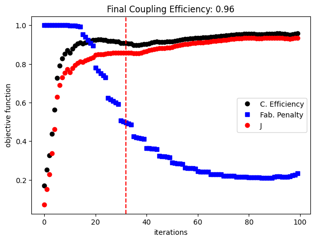
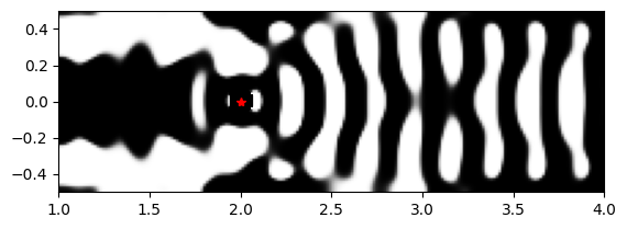
Interestingly, fully binarizing the design from iteration 32 produced a device with great coupling efficiency (~97%), but minimal purcell enhancement

plt.plot([np.linalg.norm(grad) for grad in history_dict["gradients"]])
plt.ylabel("norm(grad)")
plt.xlabel("iteration")

Text(0.5, 0, 'iteration')

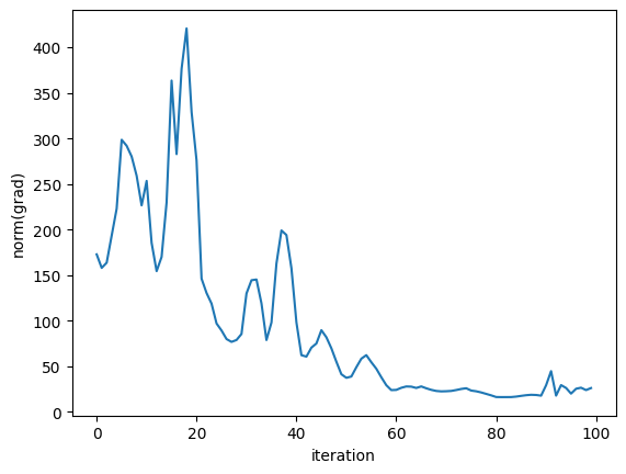
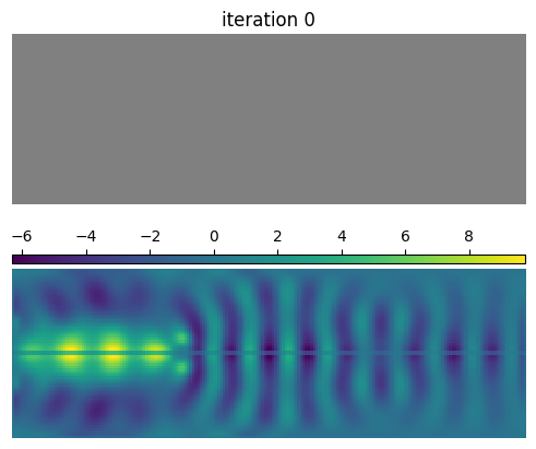
Makes a nice animation of the design parameters and gradient evolution during the optimization

import matplotlib.animation as animation
from mpl_toolkits.axes_grid1 import make_axes_locatable

fig, axs = plt.subplots(nrows=2, ncols=1)

gradients = history_dict["gradients"]
params = history_dict["params"]
gradients = [unfold_params(grad).T for grad in gradients]
params = [unfold_params(init_par).T] + [unfold_params(1.0 - p).T for p in params]

div = make_axes_locatable(axs[1])
div0 = make_axes_locatable(axs[0])
cax = div.append_axes("top", size="5%", pad=0.05)
cax0 = div0.append_axes("bottom", size="5%", pad=0.05)
cax0.axis("off")


def animate(i):
    im_g = axs[1].imshow(
        gradients[i], interpolation="none", vmin=np.min(gradients[i]), vmax=np.max(gradients[i])
    )
    axs[0].imshow(params[i], interpolation="none", cmap="gray", vmin=0, vmax=1)
    axs[1].axis("off")
    axs[0].axis("off")
    cax.cla()
    fig.colorbar(im_g, cax=cax, orientation="horizontal").ax.xaxis.set_ticks_position("top")

    axs[0].set_title(f"iteration {i}")


anim = animation.FuncAnimation(fig, animate, frames=100, blit=False, interval=500)
anim.save("autograd_anim.mp4", fps=2.0)

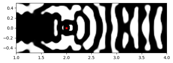
Interestingly, the final quantum emitter light extractor resembles a nanocavity, even though we have considered only the coupling efficiency into the output waveguide in the optimization. We have DBR mirrors on both sides of the dipole. However, on the left side, the mirror has only a few periods and partially reflects the radiation, which couples to the output waveguide.

# here, removing substrate improved performance, but also blue-shifted cavity resonance a bit.

fig, ax = plt.subplots(1, figsize=(10, 4))
# Substrate layer.
substrate = td.Structure(
    geometry=td.Box.from_bounds(
        rmin=(-eff_inf, -eff_inf, -eff_inf), rmax=(eff_inf, eff_inf, -wg_thick / 2)
    ),
    medium=td.Medium(permittivity=1.0),
)
sim_final = make_adjoint_sim(params2, beta=final_beta, unfold=True)
sim_final = sim_final.updated_copy(monitors=[field_monitor_xy, mode_monitor] + field_monitor)
sim_final.plot_eps(
    z=0,
    source_alpha=0,
    monitor_alpha=0,
    ax=ax,
)
plt.show()

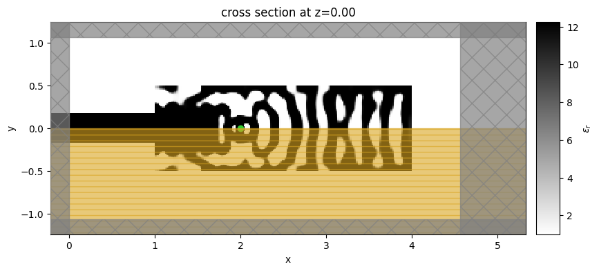
To better understand the resultant design, let’s simulate the final structure to obtain its spectral response and field distribution.

sim_data_final = web.run(sim_final, task_name="final QE light extractor")

18:56:12 CEST Created task 'final QE light extractor' with task_id
              'fdve-7b5a7f2b-9dda-46bc-8519-0af1e82273c8' and task_type 'FDTD'.

              View task using web UI at
              'https://tidy3d.simulation.cloud/workbench?taskId=fdve-7b5a7f2b-9d
              da-46bc-8519-0af1e82273c8'.

              Task folder: 'default'.

18:56:14 CEST Maximum FlexCredit cost: 0.058. Minimum cost depends on task
              execution details. Use 'web.real_cost(task_id)' to get the billed
              FlexCredit cost after a simulation run.

18:56:15 CEST status = queued

              To cancel the simulation, use 'web.abort(task_id)' or
              'web.delete(task_id)' or abort/delete the task in the web UI.
              Terminating the Python script will not stop the job running on the
              cloud.

18:56:27 CEST starting up solver

              running solver

18:56:36 CEST early shutoff detected at 24%, exiting.

              status = postprocess

18:56:41 CEST status = success

18:56:43 CEST View simulation result at
              'https://tidy3d.simulation.cloud/workbench?taskId=fdve-7b5a7f2b-9d
              da-46bc-8519-0af1e82273c8'.

18:56:47 CEST loading simulation from simulation_data.hdf5

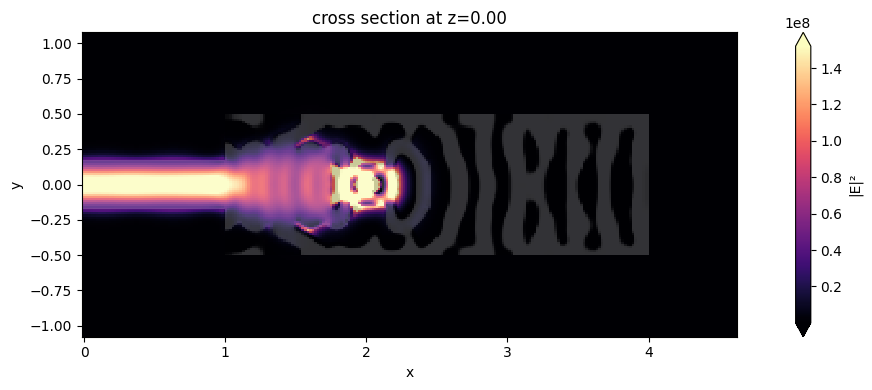
In this cavity-like system, the extraction efficiency of photons from the QE into the collection waveguide mode is proportional to \(\beta\times C_{wg}\), where the \(\beta\)-factor quantifies the fraction of the QE spontaneous emission emitted in the cavity mode, and \(C_{wg}\) is the fraction of the cavity photons coupled to the guided mode A. Enderlin, Y. Ota, R. Ohta, N. Kumagai, S. Ishida, S. Iwamoto, and Y. Arakawa, "High guided mode–cavity mode coupling for an efficient extraction of spontaneous emission of a single quantum dot embedded in a photonic crystal nanobeam cavity," Phys. Rev. B 86, 075314 (2012) DOI: 10.1103/PhysRevB.86.075314. By the field distribution image below, we can see a cavity mode resonance, which should increase the Purcell factor at the QE position, thus contributing to a higher \(\beta\)-factor. At the same time, the partial reflection mirror at the left side was potentially optimized to adjust \(C_{wg}\).

f, ax1 = plt.subplots(1, 1, figsize=(12, 4), tight_layout=True)
sim_data_final.plot_field("field_xy", "E", "abs^2", z=0, ax=ax1, f=freqs[0])
plt.show()

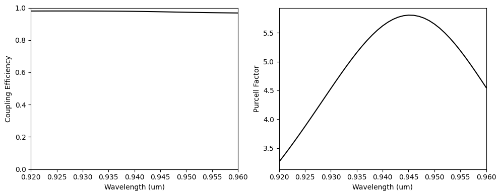
To conclude, we will calculate the final coupling efficiency and the cavity Purcell value. The coupling efficiency is above 80% along an extensive wavelength range, and we have confirmed the Purcell enhancement.

# Coupling efficiency.
mode_amps = sim_data_final["mode_monitor"].amps.sel(direction="-", mode_index=0)
mode_power = np.abs(mode_amps) ** 2
dip_power = np.zeros(n_wl)
for i in range(len(field_monitor)):
    field_mon = sim_data_final[f"field_monitor_{i}"]
    dip_power += np.abs(field_mon.flux)
coup_eff = mode_power / dip_power

# Purcell factor.
bulk_power = ((2 * np.pi * freqs) ** 2 / (12 * np.pi)) * (td.MU_0 * n_wg / td.C_0)
bulk_power = bulk_power * 2 ** (2 * np.sum(np.abs(sim_final.symmetry)))
purcell = dip_power / bulk_power

f, (ax1, ax2) = plt.subplots(1, 2, figsize=(10, 4), tight_layout=True)
ax1.plot(wl_range, coup_eff, "-k")
ax1.set_xlabel("Wavelength (um)")
ax1.set_ylabel("Coupling Efficiency")
ax1.set_ylim(0, 1)
ax1.set_xlim(wl - bw / 2, wl + bw / 2)
ax2.plot(wl_range, purcell, "-k")
ax2.set_xlabel("Wavelength (um)")
ax2.set_ylabel("Purcell Factor")
ax2.set_xlim(wl - bw / 2, wl + bw / 2)
plt.show()

print(np.max(coup_eff.values))
print(np.min(coup_eff.values))

0.9685581762335904
0.8529465434212032

Export to GDS

The Simulation object has the .to_gds_file convenience function to export the final design to a GDS file. In addition to a file name, it is necessary to set a cross-sectional plane (z = 0 in this case) on which to evaluate the geometry, a frequency to evaluate the permittivity, and a permittivity_threshold to define the shape boundaries in custom mediums. See the GDS export notebook for a detailed example on using .to_gds_file and other GDS related functions.

# make the misc/ directory to store the GDS file if it doesn't exist already
import os

if not os.path.exists("./misc/"):
    os.mkdir("./misc/")

sim_final.to_gds_file(
    fname="./misc/inv_des_light_extractor_autograd.gds",
    z=0,
    permittivity_threshold=(eps_max + eps_min) / 2,
    frequency=freq,
)