Diffractive metasurface inverse design with topology optimization#
In this tutorial, we will use inverse design and topology optimization to design a diffractive metasurface that generates a desired intensity pattern when light is transmitted through it. We use the adjoint plugin from Tidy3D to perform gradient based optimization of a mask to minimize the difference between the measured and target intensity distribution.
With Tidy3D’s adjoint plugin, we can optimize objective functions that involve arbitrary functions over measured field patterns. We define our metasurface using an arbitrary permittivity distribution as a function of (x,y) and minimize the loss function with respect to this pattern. We also include a penalty for small feature sizes.
To install the
jaxmodule required for this feature, we recommend runningpip install "tidy3d[jax]". You will also need topip install sax.
If you are unfamiliar with inverse design, we also recommend our intro to inverse design tutorials and our primer on automatic differentiation with tidy3d. For another example of metalens adjoint optimization in Tidy3D, see this example.
[1]:
import jax
import jax.numpy as jnp
import matplotlib.pyplot as plt
import numpy as np
import tidy3d as td
import tidy3d.plugins.adjoint as tda
Setup#
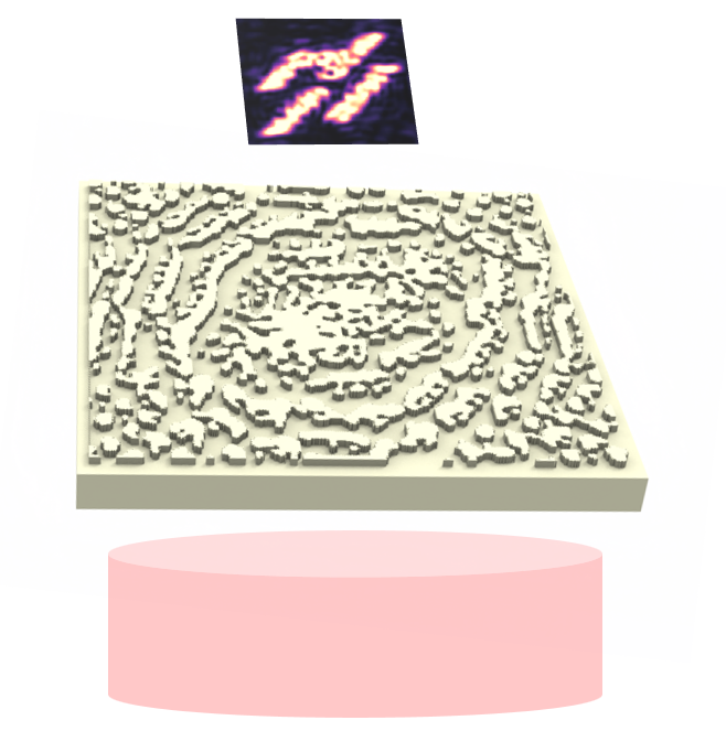
The setup is simple and similar to other examples, such as our metalens. Our structure consists of a slab of dielectric in the xy plane sitting on a substrate. A plane wave is incident from below (-z). We define the slab using a custom medium, which gives us full control of the permittivity value at each point in space.
Set Global Parameters#
[2]:
# wavelength and source properties
wavelength = 1.0
freq0 = td.C_0 / wavelength
fwidth = freq0 / 10
run_time = 100 / fwidth

# permittivity of the mask and substrate
permittivity = 2.0

# side length on x and y
length = 20

# thickness of the metalens, enough to apply a relative phase shift of just over pi
k0 = 2 * np.pi / wavelength
delta_n = np.sqrt(permittivity) - 1
thickness = 4 / k0 / delta_n

# distances between PML and source / monitor
buffer = 1.5 * wavelength

# distances between source / monitor and the mask
dist_src = 1.5 * wavelength
dist_mnt = 6.1 * wavelength

# resolution
min_steps_per_wvl = 17
[3]:
# total z size and the center of the slab
Lz = buffer + dist_src + thickness + dist_mnt + buffer
z_center_slab = -Lz / 2 + buffer + dist_src + thickness / 2.0
[4]:
# resolution of the design region
dl_design_region = 2 * wavelength / min_steps_per_wvl / np.sqrt(permittivity)

# number of pixel cells in the design region (in x and y)
nx = ny = int(length / dl_design_region)
Define Simulation Components#
We start with defining some “static” components, which don’t depend on our design parameters.
[5]:
# substrate of the same permittivity as the mask
substrate = td.Structure(
    geometry=td.Box.from_bounds(
        rmin=(-td.inf, -td.inf, -1000), rmax=(+td.inf, +td.inf, z_center_slab - thickness / 2)
    ),
    medium=td.Medium(permittivity=permittivity),
)

# plane wave
src = td.PlaneWave(
    center=(0, 0, -Lz / 2 + buffer),
    size=(td.inf, td.inf, 0),
    source_time=td.GaussianPulse(freq0=freq0, fwidth=fwidth),
    direction="+",
)

# monitor we use to measure the intensity pattern above the device
mnt_out = td.FieldMonitor(
    center=(0, 0, +Lz / 2 - buffer),
    size=(td.inf, td.inf, 0),
    freqs=[freq0],
    colocate=False,
    name="output",
)

# monitor we use to inspect the field pattern from the side for visualization
mnt_side = td.FieldMonitor(
    center=(0, 0, 0),
    size=(td.inf, 0, td.inf),
    freqs=[freq0],
    name="side",
)
Next we define the mask as a function of our design parameters using topology optimization + filtering and thresholding methods.
[6]:
from tidy3d.plugins.adjoint.utils.filter import BinaryProjector, ConicFilter

radius = 0.20
beta = 50

conic_filter = ConicFilter(radius=radius, design_region_dl=dl_design_region)


def filter_project(params: jnp.ndarray, beta: float, eta=0.5) -> jnp.ndarray:
    """Apply conic filter and binarization to the raw params."""
    params_smooth = conic_filter.evaluate(params)
    binary_projector = BinaryProjector(vmin=0, vmax=1, beta=beta, eta=eta)
    params_smooth_binarized = binary_projector.evaluate(params_smooth)
    return params_smooth_binarized


def get_eps(params: jnp.ndarray, beta: float) -> jnp.ndarray:
    """Get the permittivity values (1, permittivity) array as a function of the parameters (0, 1)"""
    mask = filter_project(params, beta)
    eps = 1 + mask * (permittivity - 1)
    return eps.reshape((nx, ny, 1, 1))


def make_slab(params: jnp.ndarray, beta: float) -> tda.JaxStructure:
    """make the phase mask as a function of the parameters for a given `beta` value."""

    # construct the coordinates
    x0_max = +length / 2 - dl_design_region / 2
    y0_max = +length / 2 - dl_design_region / 2
    coords_x = np.linspace(-x0_max, x0_max, nx).tolist()
    coords_y = np.linspace(-y0_max, y0_max, ny).tolist()
    coords = dict(x=coords_x, y=coords_y, z=[z_center_slab], f=[freq0])

    # construct the data array for the permittivity
    eps_values = get_eps(params, beta)
    eps_data_array = tda.JaxDataArray(values=eps_values, coords=coords)

    # construct the permittivity dataset
    field_components = {f"eps_{dim}{dim}": eps_data_array for dim in "xyz"}
    eps_dataset = tda.JaxPermittivityDataset(**field_components)

    # construct the phase mask slab
    custom_medium = tda.JaxCustomMedium(eps_dataset=eps_dataset)
    box = td.Box(center=(0, 0, z_center_slab), size=(td.inf, td.inf, thickness))
    return tda.JaxStructureStaticGeometry(geometry=box, medium=custom_medium)
[7]:
def make_sim(params: jnp.ndarray, beta: float, pml_xy: bool = False) -> tda.JaxSimulation:
    """The `JaxSimulation` as a function of the design parameters."""

    slab = make_slab(params, beta)

    # put a mesh override structure to ensure uniform dl across the slab
    design_region_mesh = td.MeshOverrideStructure(
        geometry=slab.geometry,
        dl=[dl_design_region] * 3,
        enforce=True,
    )

    return tda.JaxSimulation(
        size=(length, length, Lz),
        grid_spec=td.GridSpec.auto(
            min_steps_per_wvl=min_steps_per_wvl, override_structures=[design_region_mesh]
        ),
        boundary_spec=td.BoundarySpec.pml(x=pml_xy, y=pml_xy, z=True),
        input_structures=[slab],
        structures=[substrate],
        output_monitors=[mnt_out],
        monitors=[mnt_side],
        sources=[src],
        run_time=run_time,
    )
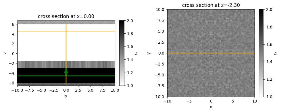
Let’s make a simulation with some random starting parameters to inspect our setup.
[8]:
params0 = np.random.random((nx, ny))
beta0 = 1.0

symmetrize = True

# symmetrize the starting parameters (optional)
if symmetrize:
    params0 += np.fliplr(params0)
    params0 += np.flipud(params0)
    params0 /= 4.0

sim = make_sim(params=params0, beta=beta0)
[9]:
f, (ax1, ax2) = plt.subplots(1, 2, figsize=(10, 4), tight_layout=True)
ax1 = sim.plot_eps(x=0, ax=ax1)
ax2 = sim.plot_eps(z=z_center_slab, ax=ax2)
plt.show()
Define Objective#
We’ll design this phase mask to give a transmitted intensity distribution of our choice.
Define Target Intensity#
In this case, we’ll try to reproduce the Flexcompute logo, so let’s make a function to generate that.
[10]:
import cv2
import xarray as xr

logo_fname = "misc/logo.png"


def get_logo() -> np.ndarray:
    """Get the Flexcompute logo from file, load it into a numpy array, rescale it to (0, 1)."""
    im = cv2.imread(logo_fname, cv2.IMREAD_GRAYSCALE).astype(float)
    im -= np.min(im)
    im /= np.max(im)
    return im


def intensity_desired_fn_logo(xs: list, ys: list, rescale: float = 0.5) -> np.ndarray:
    """Return the 'value' of the flexcompute logo as a function of (x,y) with some rescaling."""
    logo_values = get_logo()

    # some rotations to get the logo in the right orientation for the final intensity pattern
    logo_values = np.rot90(np.rot90(np.rot90(logo_values)))

    # re-interpolate the logo data at the supplied x,y points using xarray
    nx, ny = logo_values.shape
    xs_logo = np.linspace(rescale * min(xs), rescale * max(xs), nx)
    ys_logo = np.linspace(rescale * min(ys), rescale * max(ys), ny)
    logo_dataarray = xr.DataArray(logo_values, coords=dict(x=xs_logo, y=ys_logo))
    logo_interp = logo_dataarray.interp(x=xs, y=ys)

    # handle any nans for out of bounds (replace with 0)
    return np.nan_to_num(logo_interp.values, nan=np.min(logo_interp))
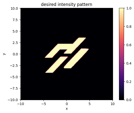
Let’s test this function out by plotting our target intensity.
[11]:
xs = ys = np.linspace(-length / 2, length / 2, nx)
intensity_desired = intensity_desired_fn_logo(xs, ys)
[12]:
plt.pcolormesh(xs, ys, intensity_desired.T, cmap="magma")
plt.gca().set_aspect("equal")
plt.xlabel("x")
plt.ylabel("y")
plt.title("desired intensity pattern")
plt.colorbar()
plt.show()
Compare Measurement to Target#
Next we need a way to compare the measured intensity pattern to this target intensity pattern.
We’ll come up with a figure of merit for the closeness of our objective.
First, let’s run a simulation with an empty mask to figure out what the average intensity should be at the measurement plane (for normalization later).
Note: Although Tidy3D normalizes field values by default, in this case doing a normalization run is useful as we’re injecting from a substrate, which will affect the results. In the new caching feature of 2.6, these simulations will not use credits or much time when run after the first time.
[13]:
params_empty = np.zeros_like(params0)

sim_empty = make_sim(params_empty, beta=100)
sim_data_norm = tda.web.run(sim_empty, task_name="normalization", verbose=True)
intensity_norm = sim_data_norm.get_intensity(mnt_out.name)
intensity_norm_mean = jnp.mean(intensity_norm.values)
15:02:14 EST Created task 'normalization' with task_id
             'fdve-e6d53724-7ff3-4d01-a5b9-072d5efbf33a' and task_type 'FDTD'.
             View task using web UI at
             'https://tidy3d.simulation.cloud/workbench?taskId=fdve-e6d53724-7ff
             3-4d01-a5b9-072d5efbf33a'.
15:02:16 EST status = success
15:02:17 EST loading simulation from simulation_data.hdf5
[14]:
print(f"Average intensity of '{intensity_norm_mean:.2f}' (a.u.) measured without any device.")
Average intensity of '1.80' (a.u.) measured without any device.
Next let’s write our loss function over the measured intensity data.
[15]:
def get_intensities(sim_data: tda.JaxSimulationData) -> tuple[jnp.ndarray, np.ndarray]:
    """Convenience function to grab the (unnormalized) intensity patterns from the data."""

    # first, grab the dataset storing the intensity values and coordinates
    intensity_dataset = sim_data.get_intensity(mnt_out.name)
    xs = intensity_dataset.coords["x"]
    ys = intensity_dataset.coords["y"]

    # the "measured" values are just the raw data
    intensity_measured = jnp.squeeze(intensity_dataset.values)

    # the "desired" or "target" values are the logo function evaluated at the data coords
    intensity_desired = intensity_desired_fn_logo(xs, ys)

    return intensity_measured, intensity_desired


# range within which to consider intensity as part of the objective function
# eg. if the measured intensity is above int_max, we just consider it at the target value of 1.0
intensity_range = int_min, int_max = (0.0, 1.0)


def intensity_diff_fn(sim_data: tda.JaxSimulationData) -> float:
    """Returns a measure for the amount of difference between desired and target intensity patterns."""

    intensity_measured, intensity_desired = get_intensities(sim_data)

    # normalize the measured intensity such that there's the same "power" in the signal as expected in the logo
    intensity_measured *= np.mean(intensity_desired) / intensity_norm_mean

    # apply the "capping" within intensity_range (optional)
    int_range_magnitude = abs(int_max - int_min)
    intensity_measured = jnp.minimum(intensity_measured, int_max)
    intensity_measured = jnp.maximum(intensity_measured, int_min)
    intensity_desired = int_range_magnitude * intensity_desired + int_min

    # take the elementwise difference
    difference = intensity_measured - intensity_desired

    # normalized by the 'worst case' (difference if measured was exact inverse of the target)
    difference_denominator = int_range_magnitude * np.ones_like(intensity_desired)

    # return the normalized norm of the difference
    return jnp.linalg.norm(difference) / jnp.linalg.norm(difference_denominator)
Fabrication Constraints#
If desired, we can add a fabrication constraint penalty to the figure of merit.
As in other notebooks, we can consider a simple penalty based on whether the structure changes upon dilation and erosion with a given distance.
[16]:
from tidy3d.plugins.adjoint.utils.penalty import ErosionDilationPenalty


def penalty_fn(params, beta):
    processed_params = filter_project(params, beta=beta)

    penalty = ErosionDilationPenalty(pixel_size=dl_design_region, length_scale=radius)
    return penalty.evaluate(processed_params)
Loss Function#
Finally, we can throw all of this into a loss function to minimize.
We will use a very small weight on our penalty function as it turns out to not be super important in this problem.
[17]:
penalty_weight = 0.1

# let's ignore the penalty for the demo, but set to True to explore how it changes the final device
include_penalty = False


def loss_fn(params: jnp.ndarray, beta: float) -> tuple[float, dict]:
    """Loss function for the design, the difference in intensity + the feature size penalty."""

    # construct and run the simulation
    sim = make_sim(params, beta=beta)
    sim_data = tda.web.run(sim, task_name="phase_mask_example", verbose=False)

    # grab the respective and total losses
    intensity_diff_loss = intensity_diff_fn(sim_data)
    if include_penalty:
        penalty_loss = penalty_weight * penalty_fn(params, beta)
    else:
        penalty_loss = 0.0

    total_loss = intensity_diff_loss + penalty_loss

    # dictionary to stash results if we want to use them in the optimization loop
    aux_data = dict(intensity_diff=intensity_diff_loss, penalty=penalty_loss, sim_data=sim_data)

    return total_loss, aux_data
Before optimizing, let’s test out our loss function to ensure we can run it and get the gradient of it with respect to the starting parameters.
[18]:
# construct a function of `params` and `beta` that returns the loss value, gradient, and the aux_data
loss_fn_val_grad = jax.value_and_grad(loss_fn, has_aux=True)

# call this on our initial parameters
(val, aux_data), grad = loss_fn_val_grad(params0, beta=beta0)
[19]:
penalty = aux_data["penalty"]
intensity_diff = aux_data["intensity_diff"]

print(f"initial loss value = {val:.3f}")
print(f" - penalty contribution = {penalty:.3f}")
print(f" - intensity difference contribution = {intensity_diff:.3f}")
print(f"gradient shape = {grad.shape:}")
print(f"norm of gradient = {jnp.linalg.norm(grad):.3e}")
initial loss value = 0.246
 - penalty contribution = 0.000
 - intensity difference contribution = 0.246
gradient shape = (239, 239)
norm of gradient = 5.256e-04
Looks good! We get a reasonable loss value, our gradient has the expected shape, and it’s non-zero (which can often indicate some issue concerning the flow of the gradient through the objective function.
Note: we passed
has_aux=True, which means that we telljaxthat the 2nd return value (aux_data) should be ignored in the gradient calculation. In other words, it tellsjaxto only consider the gradient w.r.t. the first output (total_loss).
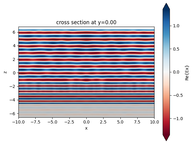
Let’s also visualize the fields for another sanity check, which we can grab from the aux_data.
[20]:
sim_data = aux_data["sim_data"]
sim_data.plot_field(field_monitor_name="side", field_name="Ex", val="real")

plt.show()
Optimize Device#
Now we are finally ready to optimize our device.
As in the other tutorials, we use the implementation of “Adam Optimization” from optax.
[21]:
import optax

# hyperparameters
num_steps = 35
learning_rate = 0.75

# initialize adam optimizer with starting parameters
params = params0.copy()
optimizer = optax.adam(learning_rate=learning_rate)
opt_state = optimizer.init(params)

# store history
history = dict(loss=[], params=[], betas=[], penalty=[], intensity_diff=[], sim_data=[])

# gradually increase the binarization strength over iteration
beta_increment = 0.5
beta = beta0

for i in range(num_steps):
    print(f"step = ({i + 1} / {num_steps})")

    # compute gradient and current loss function value
    (loss, aux_data), gradient = loss_fn_val_grad(params, beta=beta)
    penalty = aux_data["penalty"]
    intensity_diff = aux_data["intensity_diff"]

    # save history
    history["loss"].append(loss)
    history["params"].append(params)
    history["betas"].append(beta)
    history["penalty"].append(penalty)
    history["intensity_diff"].append(intensity_diff)
    history["sim_data"].append(aux_data["sim_data"])

    # log some output
    print(f"\tloss = {loss:.3e}")
    print(f"\t\tpenalty = {penalty:.3e}")
    print(f"\t\tintensity difference = {intensity_diff:.3e}")
    print(f"\tbeta = {beta:.2f}")
    print(f"\t|gradient| = {np.linalg.norm(gradient):.3e}")

    # compute and apply updates to the optimizer based on gradient (+1 sign to minimize loss_fn)
    updates, opt_state = optimizer.update(+gradient, opt_state, params)
    params = optax.apply_updates(params, updates)

    # cap the parameters between their bounds
    params = jnp.minimum(params, 1.0)
    params = jnp.maximum(params, 0.0)

    # update the beta value
    beta += beta_increment
step = (1 / 35)
        loss = 2.462e-01
                penalty = 0.000e+00
                intensity difference = 2.462e-01
        beta = 1.00
        |gradient| = 5.256e-04
step = (2 / 35)
        loss = 2.360e-01
                penalty = 0.000e+00
                intensity difference = 2.360e-01
        beta = 1.50
        |gradient| = 5.485e-04
step = (3 / 35)
        loss = 2.072e-01
                penalty = 0.000e+00
                intensity difference = 2.072e-01
        beta = 2.00
        |gradient| = 5.432e-04
step = (4 / 35)
        loss = 1.954e-01
                penalty = 0.000e+00
                intensity difference = 1.954e-01
        beta = 2.50
        |gradient| = 7.228e-04
step = (5 / 35)
        loss = 1.851e-01
                penalty = 0.000e+00
                intensity difference = 1.851e-01
        beta = 3.00
        |gradient| = 7.682e-04
step = (6 / 35)
        loss = 1.715e-01
                penalty = 0.000e+00
                intensity difference = 1.715e-01
        beta = 3.50
        |gradient| = 6.317e-04
step = (7 / 35)
        loss = 1.647e-01
                penalty = 0.000e+00
                intensity difference = 1.647e-01
        beta = 4.00
        |gradient| = 5.940e-04
step = (8 / 35)
        loss = 1.573e-01
                penalty = 0.000e+00
                intensity difference = 1.573e-01
        beta = 4.50
        |gradient| = 5.117e-04
step = (9 / 35)
        loss = 1.522e-01
                penalty = 0.000e+00
                intensity difference = 1.522e-01
        beta = 5.00
        |gradient| = 4.715e-04
step = (10 / 35)
        loss = 1.473e-01
                penalty = 0.000e+00
                intensity difference = 1.473e-01
        beta = 5.50
        |gradient| = 4.025e-04
step = (11 / 35)
        loss = 1.440e-01
                penalty = 0.000e+00
                intensity difference = 1.440e-01
        beta = 6.00
        |gradient| = 3.987e-04
step = (12 / 35)
        loss = 1.407e-01
                penalty = 0.000e+00
                intensity difference = 1.407e-01
        beta = 6.50
        |gradient| = 3.029e-04
step = (13 / 35)
        loss = 1.381e-01
                penalty = 0.000e+00
                intensity difference = 1.381e-01
        beta = 7.00
        |gradient| = 2.705e-04
step = (14 / 35)
        loss = 1.357e-01
                penalty = 0.000e+00
                intensity difference = 1.357e-01
        beta = 7.50
        |gradient| = 2.266e-04
step = (15 / 35)
        loss = 1.338e-01
                penalty = 0.000e+00
                intensity difference = 1.338e-01
        beta = 8.00
        |gradient| = 2.234e-04
step = (16 / 35)
        loss = 1.320e-01
                penalty = 0.000e+00
                intensity difference = 1.320e-01
        beta = 8.50
        |gradient| = 1.928e-04
step = (17 / 35)
        loss = 1.305e-01
                penalty = 0.000e+00
                intensity difference = 1.305e-01
        beta = 9.00
        |gradient| = 2.003e-04
step = (18 / 35)
        loss = 1.291e-01
                penalty = 0.000e+00
                intensity difference = 1.291e-01
        beta = 9.50
        |gradient| = 1.882e-04
step = (19 / 35)
        loss = 1.278e-01
                penalty = 0.000e+00
                intensity difference = 1.278e-01
        beta = 10.00
        |gradient| = 1.684e-04
step = (20 / 35)
        loss = 1.268e-01
                penalty = 0.000e+00
                intensity difference = 1.268e-01
        beta = 10.50
        |gradient| = 1.960e-04
step = (21 / 35)
        loss = 1.258e-01
                penalty = 0.000e+00
                intensity difference = 1.258e-01
        beta = 11.00
        |gradient| = 2.067e-04
step = (22 / 35)
        loss = 1.247e-01
                penalty = 0.000e+00
                intensity difference = 1.247e-01
        beta = 11.50
        |gradient| = 1.569e-04
step = (23 / 35)
        loss = 1.239e-01
                penalty = 0.000e+00
                intensity difference = 1.239e-01
        beta = 12.00
        |gradient| = 1.578e-04
step = (24 / 35)
        loss = 1.231e-01
                penalty = 0.000e+00
                intensity difference = 1.231e-01
        beta = 12.50
        |gradient| = 1.479e-04
step = (25 / 35)
        loss = 1.224e-01
                penalty = 0.000e+00
                intensity difference = 1.224e-01
        beta = 13.00
        |gradient| = 1.955e-04
step = (26 / 35)
        loss = 1.220e-01
                penalty = 0.000e+00
                intensity difference = 1.220e-01
        beta = 13.50
        |gradient| = 1.990e-04
step = (27 / 35)
        loss = 1.212e-01
                penalty = 0.000e+00
                intensity difference = 1.212e-01
        beta = 14.00
        |gradient| = 1.866e-04
step = (28 / 35)
        loss = 1.207e-01
                penalty = 0.000e+00
                intensity difference = 1.207e-01
        beta = 14.50
        |gradient| = 2.336e-04
step = (29 / 35)
        loss = 1.201e-01
                penalty = 0.000e+00
                intensity difference = 1.201e-01
        beta = 15.00
        |gradient| = 2.416e-04
step = (30 / 35)
        loss = 1.196e-01
                penalty = 0.000e+00
                intensity difference = 1.196e-01
        beta = 15.50
        |gradient| = 2.157e-04
step = (31 / 35)
        loss = 1.191e-01
                penalty = 0.000e+00
                intensity difference = 1.191e-01
        beta = 16.00
        |gradient| = 2.127e-04
step = (32 / 35)
        loss = 1.186e-01
                penalty = 0.000e+00
                intensity difference = 1.186e-01
        beta = 16.50
        |gradient| = 2.165e-04
step = (33 / 35)
        loss = 1.184e-01
                penalty = 0.000e+00
                intensity difference = 1.184e-01
        beta = 17.00
        |gradient| = 2.566e-04
step = (34 / 35)
        loss = 1.182e-01
                penalty = 0.000e+00
                intensity difference = 1.182e-01
        beta = 17.50
        |gradient| = 2.685e-04
step = (35 / 35)
        loss = 1.180e-01
                penalty = 0.000e+00
                intensity difference = 1.180e-01
        beta = 18.00
        |gradient| = 3.073e-04
Analyze Results#
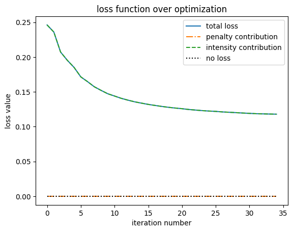
First, let’s plot the objective function history.
[22]:
plt.plot(history["loss"], label="total loss")
plt.plot(history["penalty"], linestyle="-.", label="penalty contribution")
plt.plot(history["intensity_diff"], linestyle="--", label="intensity contribution")
plt.plot(np.zeros_like(history["loss"]), linestyle=":", color="k", label="no loss")

plt.xlabel("iteration number")
plt.ylabel("loss value")

plt.title("loss function over optimization")
plt.legend()
plt.show()
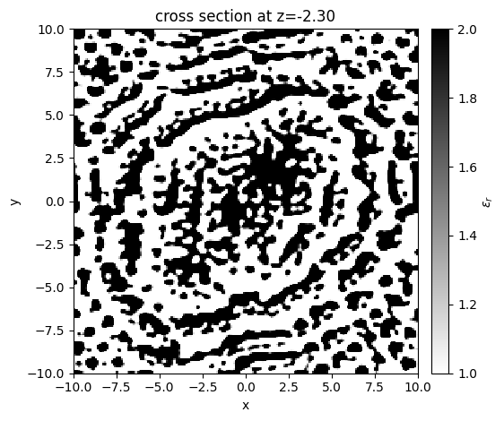
Next let’s plot the final device pattern.
[23]:
# get the final parameters, construct the final simulation
params_final = history["params"][-1]
beta_final = history["betas"][-1]
jax_sim_final = make_sim(params_final, beta=beta_final)

# convert to regular `td.Simulation`
sim_final = jax_sim_final.to_simulation()[0]
sim_final.plot_eps(z=z_center_slab, monitor_alpha=0)

plt.show()
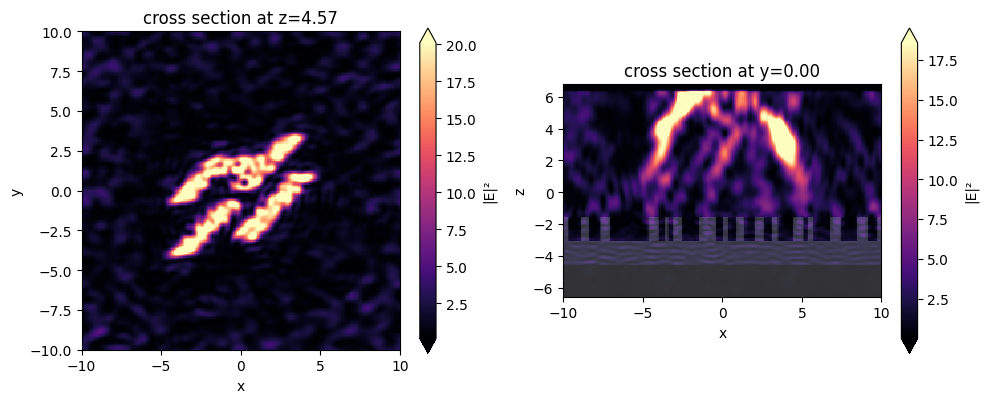
Let’s run this simulation to see the final field patterns
[24]:
sim_data_final = td.web.run(sim_final, task_name="Inspect")
17:07:52 EST Created task 'Inspect' with task_id
             'fdve-80edc529-81fc-4a35-90bf-f8aeaaef4c54' and task_type 'FDTD'.
             View task using web UI at
             'https://tidy3d.simulation.cloud/workbench?taskId=fdve-80edc529-81f
             c-4a35-90bf-f8aeaaef4c54'.
17:07:56 EST status = queued
17:08:04 EST status = preprocess
17:08:07 EST Maximum FlexCredit cost: 0.127. Use 'web.real_cost(task_id)' to get
             the billed FlexCredit cost after a simulation run.
starting up solver
running solver
             To cancel the simulation, use 'web.abort(task_id)' or
             'web.delete(task_id)' or abort/delete the task in the web UI.
             Terminating the Python script will not stop the job running on the
             cloud.
17:09:16 EST early shutoff detected at 96%, exiting.
status = postprocess
17:09:23 EST status = success
             View simulation result at
             'https://tidy3d.simulation.cloud/workbench?taskId=fdve-80edc529-81f
             c-4a35-90bf-f8aeaaef4c54'.
17:09:25 EST loading simulation from simulation_data.hdf5
[25]:
f, axes = plt.subplots(1, 2, figsize=(10, 4), tight_layout=True)

for ax, name in zip(axes, ("output", "side")):
    sim_data_final.plot_field(field_monitor_name=name, field_name="E", val="abs^2", ax=ax)
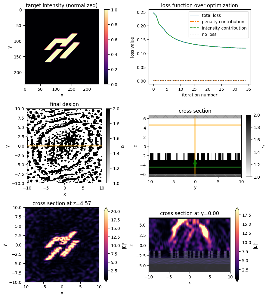
Finally, we can create a nice figure combining everything.
[26]:
f, ((ax0, ax1), (ax2, ax3), (ax4, ax5)) = plt.subplots(3, 2, figsize=(9, 10), tight_layout=True)

# target intensity
im = ax0.imshow(np.rot90(intensity_desired), cmap="magma")
ax0.set_aspect("equal")
ax0.set_xlabel("x")
ax0.set_ylabel("y")
ax0.set_title("target intensity (normalized)")
plt.colorbar(im, ax=ax0)

# optimization progress
ax1.plot(history["loss"], label="total loss")
ax1.plot(history["penalty"], linestyle="-.", label="penalty contribution")
ax1.plot(history["intensity_diff"], linestyle="--", label="intensity contribution")
ax1.plot(np.zeros_like(history["loss"]), linestyle=":", color="k", label="no loss")
ax1.set_xlabel("iteration number")
ax1.set_ylabel("loss value")
ax1.set_title("loss function over optimization")
ax1.legend()

# ax1.plot(history["loss"])
# ax1.set_xlabel("iterations")
# ax1.set_ylabel("loss function")
# ax1.set_title('optimization progress')

# final device (top and sides)
sim_final.plot_eps(z=z_center_slab, ax=ax2)
ax2.set_title("final design")
sim_final.plot_eps(x=0, ax=ax3)
ax3.set_title("cross section")

# final fields
vmin = None
vmax = None
for ax, name in zip((ax4, ax5), ("output", "side")):
    sim_data_final.plot_field(
        field_monitor_name=name, field_name="E", val="abs^2", vmin=vmin, vmax=vmax, ax=ax
    )

# plt.savefig('phase_mask.png', dpi=300)
plt.show()
[ ]:
[ ]: