Robust Adjoint Optimization for Manufacturability

In the previous notebook, we discovered that our apodized grating is somewhat brittle: realistic ±20 nm fabrication errors can reduce efficiency by almost a decibel. A design that only works on paper is not a practical solution.

In this final notebook we incorporate fabrication awareness directly into the adjoint optimization loop. Instead of optimizing a single, nominal simulation, we will maximize the performance across multiple fabrication corners so the resulting device maintains high efficiency even when etched dimensions shift on the wafer.

import json
from copy import deepcopy
from pathlib import Path

import autograd.numpy as np
import matplotlib.pyplot as plt
import tidy3d as td
from autograd import value_and_grad
from optim import adam_update, apply_updates, clip_params, init_adam
from setup import (
    center_wavelength,
    first_gap_sin,
    get_mode_monitor_power,
    make_simulation,
    max_gap_si,
    max_gap_sin,
    max_width_si,
    max_width_sin,
    min_gap_si,
    min_gap_sin,
    min_width_si,
    min_width_sin,
)
from tidy3d import web

ETCH_BIAS = 0.02  # 20 nm fabrication bias expressed in microns.


def apply_bias(param_dict, etch_bias):
    """Return a new parameter dictionary with widths widened by bias."""
    return {
        "widths_si": param_dict["widths_si"] + etch_bias,
        "gaps_si": param_dict["gaps_si"] - etch_bias,
        "widths_sin": param_dict["widths_sin"] + etch_bias,
        "gaps_sin": param_dict["gaps_sin"] - etch_bias,
        "first_gap_si": param_dict["first_gap_si"],
        "first_gap_sin": param_dict["first_gap_sin"],
    }

Defining a Robust Multi-Objective Function

We evaluate the design under three fabrication scenarios: nominal, over-etched (−20 nm), and under-etched (+20 nm). We then maximize the mean transmission and simultaneously minimize the standard deviation in performance between these different scenarios, which should lead to a more robust design overall. The amount of weight we place on the standard deviation minimization determines the tradeoff between nominal performance and robustness.

STD_PENALTY = 2.0  # Penalty for standard deviation in power


def robust_objective(params):
    freq0 = td.C_0 / center_wavelength
    scenarios = {
        "nominal": params,
        "over": apply_bias(params, -ETCH_BIAS),
        "under": apply_bias(params, ETCH_BIAS),
    }

    sims = {
        name: make_simulation(
            scenario["widths_si"],
            scenario["gaps_si"],
            scenario["widths_sin"],
            scenario["gaps_sin"],
            first_gap_si=scenario["first_gap_si"],
            first_gap_sin=scenario["first_gap_sin"],
        )
        for name, scenario in scenarios.items()
    }

    batch_data = web.run_async(sims, verbose=False, local_gradient=True)

    powers = []
    for name in ("nominal", "over", "under"):
        sim_data = batch_data[name]
        power_da = get_mode_monitor_power(sim_data)
        target_power = power_da.sel(f=freq0, method="nearest")
        powers.append(target_power.item())

    powers = np.array(powers)
    mean_power = np.mean(powers)
    variance = np.mean((powers - mean_power) ** 2)
    std_power = np.sqrt(variance)
    robust_metric = mean_power - STD_PENALTY * std_power

    return -robust_metric

Starting Point and Bounds

We seed the optimizer with the fabrication-sensitive adjoint design and enforce the same foundry limits as before so the updates remain manufacturable.

data = json.loads(Path("./results/gc_adjoint_best.json").read_text(encoding="utf-8"))

num_iters = 40

params0 = {
    "widths_si": np.array(data["widths_si"], dtype=float),
    "gaps_si": np.array(data["gaps_si"], dtype=float),
    "widths_sin": np.array(data["widths_sin"], dtype=float),
    "gaps_sin": np.array(data["gaps_sin"], dtype=float),
    "first_gap_si": float(data["first_gap_si"]),
    "first_gap_sin": float(data.get("first_gap_sin", first_gap_sin)),
}

bounds = {
    "widths_si": (min_width_si, max_width_si),
    "gaps_si": (min_gap_si, max_gap_si),
    "widths_sin": (min_width_sin, max_width_sin),
    "gaps_sin": (min_gap_sin, max_gap_sin),
    "first_gap_si": (None, None),
    "first_gap_sin": (min_gap_sin, None),
}

Running the Robust Optimization

Starting from the adjoint-optimized design found earlier, we use Adam to minimize the robust objective.

vg_fun = value_and_grad(robust_objective)
params = deepcopy(params0)
opt_state = init_adam(params, lr=1e-3)

objective_history = []

for n in range(num_iters):
    value, grad = vg_fun(params)
    objective_value = -value

    objective_history.append(objective_value)
    print(f"iter {n}: objective={objective_value:.4f}")

    updates, opt_state = adam_update(grad, opt_state)
    params = apply_updates(params, updates)
    params = clip_params(params, bounds)

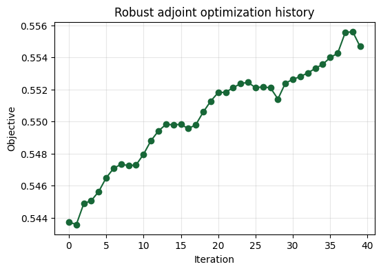
Tracking Progress

Plotting the objective over iterations lets us confirm that the robust objective steadily improves (higher is better).

fig, ax = plt.subplots(figsize=(6, 4))
ax.plot(np.arange(len(objective_history)), objective_history, marker="o")
ax.set_xlabel("Iteration")
ax.set_ylabel("Objective")
ax.set_title("Robust adjoint optimization history")
ax.grid(True, alpha=0.3)
plt.show()

Pre- and Post-Optimization Bias Sweeps

To visualize the payoff, we re-run the ±20 nm fabrication corners for the original and robust designs. This mirrors the analysis step from the sensitivity notebook so we can compare apples to apples.

def to_numpy_params(param_dict):
    """Detach autograd arrays into plain numpy arrays for analysis/export."""
    return {
        "widths_si": np.array(param_dict["widths_si"], dtype=float),
        "gaps_si": np.array(param_dict["gaps_si"], dtype=float),
        "widths_sin": np.array(param_dict["widths_sin"], dtype=float),
        "gaps_sin": np.array(param_dict["gaps_sin"], dtype=float),
        "first_gap_si": float(param_dict["first_gap_si"]),
        "first_gap_sin": float(param_dict["first_gap_sin"]),
    }


def run_bias_sweep(param_dict, task_prefix, bias=ETCH_BIAS):
    """Run nominal/over/under simulations and return spectra in linear scale."""
    scenarios = [
        ("Over-etched (-20 nm)", apply_bias(param_dict, -bias)),
        ("Nominal", param_dict),
        ("Under-etched (+20 nm)", apply_bias(param_dict, bias)),
    ]

    sims = {
        f"{task_prefix}_{idx}": make_simulation(
            scenario["widths_si"],
            scenario["gaps_si"],
            scenario["widths_sin"],
            scenario["gaps_sin"],
            first_gap_si=scenario["first_gap_si"],
            first_gap_sin=scenario["first_gap_sin"],
        )
        for idx, (_, scenario) in enumerate(scenarios)
    }

    batch_data = web.run_async(sims, verbose=False)

    wavelengths = None
    spectra = {}
    for idx, (label, _) in enumerate(scenarios):
        sim_data = batch_data[f"{task_prefix}_{idx}"]
        power_da = get_mode_monitor_power(sim_data)
        freqs = power_da.coords["f"].values
        wl = td.C_0 / freqs
        power = np.asarray(power_da.data).squeeze()
        order = np.argsort(wl)
        wl = wl[order]
        power = power[order]
        if wavelengths is None:
            wavelengths = wl
        spectra[label] = power
    return wavelengths, spectra


params_initial = to_numpy_params(params0)
params_robust = to_numpy_params(params)

w_before, spectra_before = run_bias_sweep(params_initial, "gc_robust_bias_before", bias=ETCH_BIAS)
w_after, spectra_after = run_bias_sweep(params_robust, "gc_robust_bias_after", bias=ETCH_BIAS)

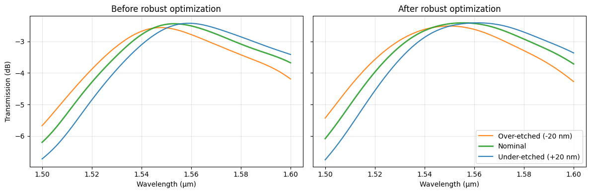
The Final Payoff: Visualizing Robustness

The left panel shows how sensitive the previous design is to ±20 nm fabrication bias, while the right panel show the spectrum after robust optimization. We can see observe a slight shift in the spectra, but to make any quantitative statement, we’ll not to run another sensitivity analysis, which we’ll do in the next notebook.

labels = ["Over-etched (-20 nm)", "Nominal", "Under-etched (+20 nm)"]
colors = {
    "Over-etched (-20 nm)": "tab:orange",
    "Nominal": "tab:green",
    "Under-etched (+20 nm)": "tab:blue",
}

fig, axes = plt.subplots(1, 2, figsize=(12, 4), sharey=True)

for label in labels:
    axes[0].plot(
        w_before,
        10 * np.log10(spectra_before[label]),
        label=label,
        color=colors[label],
        linewidth=2 if label == "Nominal" else 1.6,
        alpha=0.9,
    )

axes[0].set_title("Before robust optimization")
axes[0].set_xlabel("Wavelength (µm)")
axes[0].set_ylabel("Transmission (dB)")
axes[0].grid(True, alpha=0.3)

for label in labels:
    axes[1].plot(
        w_after,
        10 * np.log10(spectra_after[label]),
        label=label,
        color=colors[label],
        linewidth=2 if label == "Nominal" else 1.6,
        alpha=0.9,
    )

axes[1].set_title("After robust optimization")
axes[1].set_xlabel("Wavelength (µm)")
axes[1].grid(True, alpha=0.3)
axes[1].legend(loc="best")

plt.tight_layout()
plt.show()

Exporting the Robust Design

Finally we save the fabrication-aware geometry so downstream notebooks - or a GDS handoff - can reuse it without re-running the optimization loop.

export_path = Path("./results/gc_adjoint_robust_best.json")
export_payload = {
    "widths_si": params_robust["widths_si"].tolist(),
    "gaps_si": params_robust["gaps_si"].tolist(),
    "widths_sin": params_robust["widths_sin"].tolist(),
    "gaps_sin": params_robust["gaps_sin"].tolist(),
    "first_gap_si": params_robust["first_gap_si"],
    "first_gap_sin": params_robust["first_gap_sin"],
    "etch_bias_modeled": ETCH_BIAS,
}

export_path.parent.mkdir(parents=True, exist_ok=True)
export_path.write_text(json.dumps(export_payload, indent=2), encoding="utf-8")
print(f"Saved robust design to {export_path.resolve()}")

Saved robust design to /home/yannick/flexcompute/worktrees/seminar_notebooks/docs/notebooks/2025-10-09-invdes-seminar/results/gc_adjoint_robust_best.json